Introduction
Text Generation
Natural Language Processing (NLP) is a branch of artificial intelligence that is steadily growing both in terms of research and market values1. The ultimate objective of NLP is to read, decipher, understand, and make sense of the human languages in a manner that is valuable2. The are many applications of NLP in various industries, such as:
- SPAM email detection
- Sentiment Analysis
- Text summarization
- Topic Modelling
- Text Generation
In this article, we will try to learn the last one: text generation. The goal of text generation is to create a predictive text or an auto-generated text based on the previous typed term or word. The easiest example of text generation is the predictive text when you type in the search tab of Google3 or when you write an email.
Autocomplete is especially useful for those using mobile devices, making it easy to complete a search on a small screen where typing can be hard. For both mobile and desktop users, it’s a huge time saver all around.
 {width = “80%”}
Another implementation of text generation is to create an artificial text or script, which can be potentially applied to generate artificial news, create a better movie synopsis, create poems, or even create an entire book.
The following text is generated using the natural language processing model architecture called GPT-24. You can try to create one by visiting the website made by Adam King5. Text generation can also be applied for image captioning or music generation, depending on the input6.
 {width = “60%”}
GPT-2 is a very sophisticated model that use more than 8 million web pages as it training dataset. However, due to the great potential to be misused, the developers decided not to release the trained model. An alternative to create our own custom text generator is using the Recurrent Neural Network and it’s LSTM companion7. However, there is a simpler approach to create a text generator using a model called Markov Chain8. The state-of-the-art or the development of text generation can be found at Fonseca9.
Markov Chain is a mathematical model of stochastic process that predicts the condition of the next state (e.g. will it rain tomorrow?) based on the condition of the previous one. Using this principle, the Markov Chain can predict the next word based on the last word typed. Victor Powell10 has dedicated a great website to visualize how Markov Chains work.
Through this article, we will explore the mechanism behind Markov Chains and how to apply it to create a text generator and some other use cases.
Training Objective
The goal of this article is to help you:
- Understand the concept of Markov Chains
- Understand the properties of Markov Chains
- Implement Markov Chains to create a text generator
- Create Markov Chains with 1-gram, 2-gram and 3-gram text
- Implement Markov Chains in several business cases
In order to understand the topic covered here, you may at least need to understand some of the following topics:
- Basic theory of probability
- General understanding of text mining
Library and Setup
The following package is required for the next section.
# Data wrangling
library(tidyverse)

# Text processing
library(tidytext)
library(textclean)
library(tokenizers)

# Markov Chain
library(markovchain)
Markov Chain
This section is dedicated to give you a general understanding of the elements and characteristics of Markov Chains.
Transition Probability
Markov Chain is a mathematical model of stochastic process that predicts the condition of the next state based on condition of the previous state. It is called as a stochastic process because it change or evolve over time.
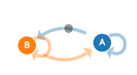
Let’s consider the following graph to illustrate what Markov Chains is.
 {width = “40%”}
From the above network, let’s say that there are two states: A (rain) and B (sunny). If today weather is in state A (rain), there are two possibilities for the next day. Tomorrow can be rain again, indicated by the circular loop (from A to A again), or tomorrow can be sunny (B). The same goes for the state B, it can go from state B to B again on the next day, or it can be rainy (A). Each transition from A to A or A to B will have it’s own probability to happen. The Markov Chain will model the probability of transition between the current state toward the next one.
For more illustrative example, let’s say we have a data of weather condition for the past 100 days.
weather <- c("sunny", "sunny", "rain", "cloudy")

set.seed(123)
weather_data <- sample(weather, 100, replace = T)
head(weather_data, 10)
#> [1] "rain" "rain" "rain" "sunny" "rain" "sunny" "sunny" "sunny" "rain"
#> [10] "sunny"table(weather_data) %>% prop.table()#> weather_data
#> cloudy rain sunny
#> 0.17 0.29 0.54If today is sunny, what is the probability that tomorrow will be sunny as well? We simply just need to calculate how many times that today is sunny and the next day is sunny as well from the data.
embed(weather_data, 2)[, 2:1] %>%
   as.data.frame() %>%
   rename(current = V1, next_day = V2) %>%
   filter(current == "sunny") %>%
   arrange(next_day) %>%
   count(current, next_day)
#> # A tibble: 3 x 3
#> current next_day n
#> <fct> <fct> <int>
#> 1 sunny cloudy 6
#> 2 sunny rain 18
#> 3 sunny sunny 30Based on the data, if current day is sunny, there are 6 occurences that the next day would be cloudy, 18 occurences that the next day is rain, and 30 occurences that the next day is sunny again. Based on the data, we can directly calculate the probability. For example, if the current day is sunny, the probability that the next day would be sunny again is:
\[P_{sunny\ sunny} = \frac{30}{30+6+18} = 0.556\]
This probability is called as the Transition Probability and represent the probability that tomorrow will be sunny if today is sunny. Below is the probability for each next state if today is sunny.
#> Probability of each weather tomorrow if today is sunny
#>    cloudy      rain     sunny
#> 0.1111111 0.3333333 0.5555556
The above probability only consider that the current state (today) is sunny. We also need to consider other condition of the current state, which includes cloudy and rain.
# Probability if today is cloudy
weather_cloudy <- embed(weather_data, 2)[, 2:1] %>%
   as.data.frame() %>%
   rename(current = V1, next_day = V2) %>%
   filter(current == "cloudy") %>%
   pull(next_day) %>%
   table("Probability of each weather tomorrow if today is cloudy" = .) %>% prop.table()


# Probability if today is rainy
weather_rain <- embed(weather_data, 2)[, 2:1] %>%
   as.data.frame() %>%
   rename(current = V1, next_day = V2) %>%
   filter(current == "rain") %>%
   pull(next_day) %>%
   table("Probability of each weather tomorrow if today is rain" = .) %>% prop.table()

weather_cloudy
#> Probability of each weather tomorrow if today is cloudy
#> cloudy rain sunny
#> 0.1176471 0.1764706 0.7058824weather_rain#> Probability of each weather tomorrow if today is rain
#> cloudy rain sunny
#> 0.3214286 0.2500000 0.4285714Transition Probability Matrix
After we have calculated all probability, we can assemble a matrix called Transition Probability Matrix. As it name suggest, the matrix consists of all transition probability from the current state toward the next state.
trans_matrix <- rbind(weather_cloudy, weather_rain, weather_sunny) %>%
   `rownames<-`(c("cloudy", "rain", "sunny"))

trans_matrix
#> cloudy rain sunny
#> cloudy 0.1176471 0.1764706 0.7058824
#> rain 0.3214286 0.2500000 0.4285714
#> sunny 0.1111111 0.3333333 0.5555556Some characteristic of the transition probability matrix:
- The transition matrix is always a square matrix or n-by-n matrix (number of rows and columns are the same)
- The dimension of transition matrix is determined by the number of all possible states
- The row (commonly) represent the current state
- The column (commonly) represent the next state
- The total probability for each current state (row) is 1
- The next/future state is only depends on the current state and independent from the past, this properties is called Lack of Memories
The markovchain package will help us to simplify many process related to Markov Chains. But first, we need to convert the trans_matrix from matrix into a markovchain object.
# convert the matrix as a markov chain object
markov_model <- new("markovchain",
transitionMatrix = trans_matrix, # Input Transition Matrix
name = "Weather") # Name of the Markov Chains
markov_model#> Weather
#> A 3 - dimensional discrete Markov Chain defined by the following states:
#> cloudy, rain, sunny
#> The transition matrix (by rows) is defined as follows:
#>           cloudy      rain     sunny
#> cloudy 0.1176471 0.1764706 0.7058824
#> rain   0.3214286 0.2500000 0.4285714
#> sunny 0.1111111 0.3333333 0.5555556The Markov Chains can be presented visually by using plot() function toward the markovchain object.
set.seed(2)
plot(markov_model)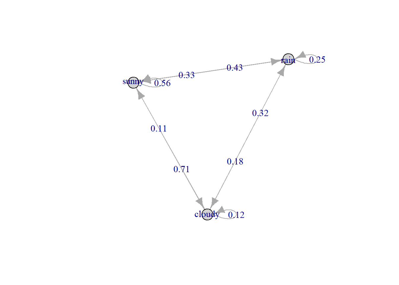
The arrow indicate the transition toward the next state while the number shows the probability of those transition. For example, there is a probability of 0.32 for transition from rain today toward cloudy tommorow. If the next state is the same as the current state, the arrow will make a loop toward itself, like the 25% probability of rain today to rain again tommorow.
Another way to create a Markov Chains without manually calculating the transition matrix is by using markovchainFit() function from the markovchain package. The function will automatically detect a sequence from the input vector and create a transition probability matrix. The only difference is that markovchainFit() use estimation method to calculate the transition probability. The default method to calculate the transition probability is by using Maximum Likelihood Method (MLE) by using the following equation:
\[\hat p_{ij} = \frac{n_{ij}}{\Sigma_{u = 1}^k n_{iu}}\]
\(\hat p_{ij}\) = transition probability from state i to state j
\(n_{ij}\) = number of sequence from i to j from the data
\(n_{iu}\) = number of sequence from i to u with \(u = 1, 2, ..., k\)
\(k\) = number of all possible states
You can also add laplace smoothing and slightly modify the equation using the laplacian method:
\[\hat p_{ij} = \frac{n_{ij} + \alpha}{\Sigma_{u = 1}^k (n_{iu}+ \alpha)}\]
\(\alpha\) = Laplace smoothing constant
We will try to create the Markov Chains using the markovchainFit() function. The transition matrix can be acquired at the estimate output from the markovchain object.
# Fit the data
markov_weather <- markovchainFit(weather_data, method = "mle")

# Get transition probaiblity
markov_weather$estimate
#> MLE Fit
#> A 3 - dimensional discrete Markov Chain defined by the following states:
#> cloudy, rain, sunny
#> The transition matrix (by rows) is defined as follows:
#> cloudy rain sunny
#> cloudy 0.1176471 0.1764706 0.7058824
#> rain 0.3214286 0.2500000 0.4285714
#> sunny 0.1111111 0.3333333 0.5555556The transition matrix is identical with the previous one.
Chapman-Kolmogorov Equation
Once again, let’s visualize the Markov Chains of the weather data.
set.seed(123)
plot(markov_weather$estimate)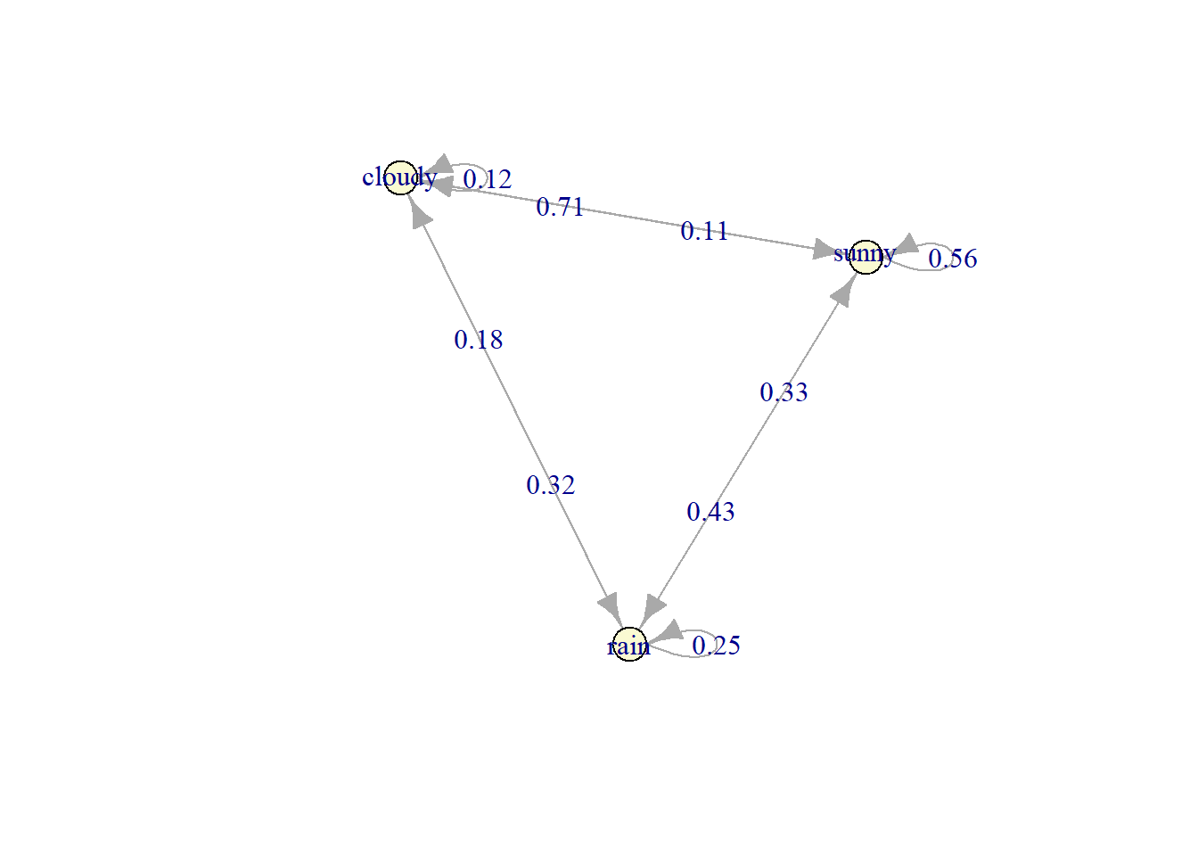
So, based on the transition matrix, if today is cloudy, the chance that tomorrow will be sunny is 71%. But what about the next 2 days? Or even the next 7 days?
The arrow indicate the transition toward the next state while the number shows the probability of those transition. For example, there is a probability of 0.32 for transition from rain today toward cloudy tommorow. If the next state is the same as the current state, the arrow will make a loop toward itself, like the 25% probability of rain today to rain again tommorow.
By using Markov Chains, we can get the transition matrix for the next n-period by simply multiply the transition matrix with itself. For example, if we want to get the transition matrix for the next 2 days:
# Matrix multiplication
markov_weather$estimate * markov_weather$estimate
#> MLE Fit
#> A 3 - dimensional discrete Markov Chain defined by the following states:
#> cloudy, rain, sunny
#> The transition matrix (by rows) is defined as follows:
#> cloudy rain sunny
#> cloudy 0.1489949 0.3001730 0.5508321
#> rain 0.1657913 0.2620798 0.5721289
#> sunny 0.1819431 0.2881264 0.5299305So, if today is cloudy, the chance that the 2 days from now is sunny is 55.08%. How can we arrive at such conclusion? This principle is called the Chapman-Kolmogorov Equation.
\[p_{ij}^{n} = \Sigma_{k=1}^{M} p_{ik}^{m}\ p_{kj}^{n-m}\]
\(p_{ij}^{n}\) = probability that the system will be at state j at the n-step if it is on the state i during m-step.
Basically, it means that in order to arrive at the sunny state at the second day, there are multiple route that can be traveled:
- today cloudy -> tomorrow sunny -> next 2 days sunny
- today cloudy -> tomorrow cloudy -> next 2 days sunny
- today cloudy -> tomorrow rain -> next 2 days sunny
The Markov Chains is often more often represented as a transition probability matrix instead of a graph, with each row indicate the current states while each column indicate the next states. Based on the previous graph, we can convert it into the following transition matrix:
We just need to calculate the probability for each routes and sum it all at the end.
Let’s go back to the initial transition matrix:
markov_weather$estimate#> MLE Fit
#> A 3 - dimensional discrete Markov Chain defined by the following states:
#> cloudy, rain, sunny
#> The transition matrix (by rows) is defined as follows:
#> cloudy rain sunny
#> cloudy 0.1176471 0.1764706 0.7058824
#> rain 0.3214286 0.2500000 0.4285714
#> sunny 0.1111111 0.3333333 0.5555556Based on the Chapman-Kolmogorov, the probability to be sunny at the next 2 days if today is cloudy is:
\[p_{cloudy\ sunny}^{2} = \Sigma_{k=0}^{3} p_{cloudy\ k}^{1}\ p_{k\ j}^{2-1}\]
\[p_{cloudy\ sunny}^{2} = p_{cloudy\ cloudy}^{1}\ p_{cloudy\ sunny}^{2-1} + p_{cloudy\ sunny}^{1}\ p_{sunny\ sunny}^{2-1}+p_{cloudy\ rain}^{1}\ p_{rain\ sunny}^{2-1}\]
\[p_{cloudy\ sunny}^{2} = 0.1176\ \ 0.7059 + 0.1765\ 0.4286+ 0.7059\ 0.5556 = 0.5509\]
Or simply
current_state <- c(1, 0, 0) # today is cloudy

current_state * markov_weather$estimate^2 # probability for the next 2 days
#> cloudy rain sunny
#> [1,] 0.1489949 0.300173 0.5508321Let’s go back to the matrix multiplication and check the result:
markov_weather$estimate * markov_weather$estimate#> MLE Fit
#> A 3 - dimensional discrete Markov Chain defined by the following states:
#> cloudy, rain, sunny
#> The transition matrix (by rows) is defined as follows:
#> cloudy rain sunny
#> cloudy 0.1489949 0.3001730 0.5508321
#> rain 0.1657913 0.2620798 0.5721289
#> sunny 0.1819431 0.2881264 0.5299305The probability from cloudy to sunny in the next 2 days is 0.5508.
For the next 7 days, we simply multiply the matrix 7 times:
markov_weather$estimate^7#> MLE Fit^7
#> A 3 - dimensional discrete Markov Chain defined by the following states:
#> cloudy, rain, sunny
#> The transition matrix (by rows) is defined as follows:
#> cloudy rain sunny
#> cloudy 0.1717223 0.2828268 0.5454509
#> rain 0.1717158 0.2828327 0.5454515
#> sunny 0.1717163 0.2828265 0.5454573So for the next 7 days, the chance of sunny if today is cloudy is 54.5%.
Special State in Markov Chains
There are at least 4 special or notable state in Markov Chains:
- Steady State
- Absorbing State
- Transient State
- Recurrent State
Understanding the presence of those stats is useful if we wish to analyze the system via Markov Chains.
Steady States
In Markov Chains, there exist a condition where regardless of the current state, the probability for the next state is always the same. Let’s check the transition Matrix for the next 14 days:
markov_weather$estimate^14#> MLE Fit^14
#> A 3 - dimensional discrete Markov Chain defined by the following states:
#> cloudy, rain, sunny
#> The transition matrix (by rows) is defined as follows:
#> cloudy rain sunny
#> cloudy 0.1717172 0.2828283 0.5454545
#> rain 0.1717172 0.2828283 0.5454545
#> sunny 0.1717172 0.2828283 0.5454545As we can see, regardless if today is cloudy, rain, or sunny, the probability that tomorrow will be sunny is always 0.545 and tomorrow will be rain is always 0.2828. This condition is called the Steady-state of the transition matrix. It means that after certain point of time/step, the probability of the next step will always be the same for each state. A steady-state is important to do a long-term analysis such as insurance, inventory management, and maintenance policy.
To get the steady-state of the Markov Chains, we simply use steadyStates() function.
steadyStates(markov_weather$estimate)#> cloudy rain sunny
#> [1,] 0.1717172 0.2828283 0.5454545Based on the result, regardless of the current weather, the probability that tomorrow will be cloudy is 0.17, tomorrow will be rain is 0.28 and tomorrow will be sunny is 0.545.
Absorbing State
Supossed that we have the following transition matrix from Health Insurance:
# create transition matrix
transition_matrix <- matrix(c(0.5, .25, .15, .1,
                              0.4, 0.4, 0.0, 0.2,
                              0, 0, 1, 0,
                              0, 0, 0, 1),
                            byrow = TRUE, nrow = 4)

# convert the matrix as a markov chain object

markov_health <- new("markovchain", transitionMatrix = transition_matrix,
                    name = "Health Insurance",
                    states = c("active", "disable", "withdrawn", "death"))

set.seed(4)
plot(markov_health)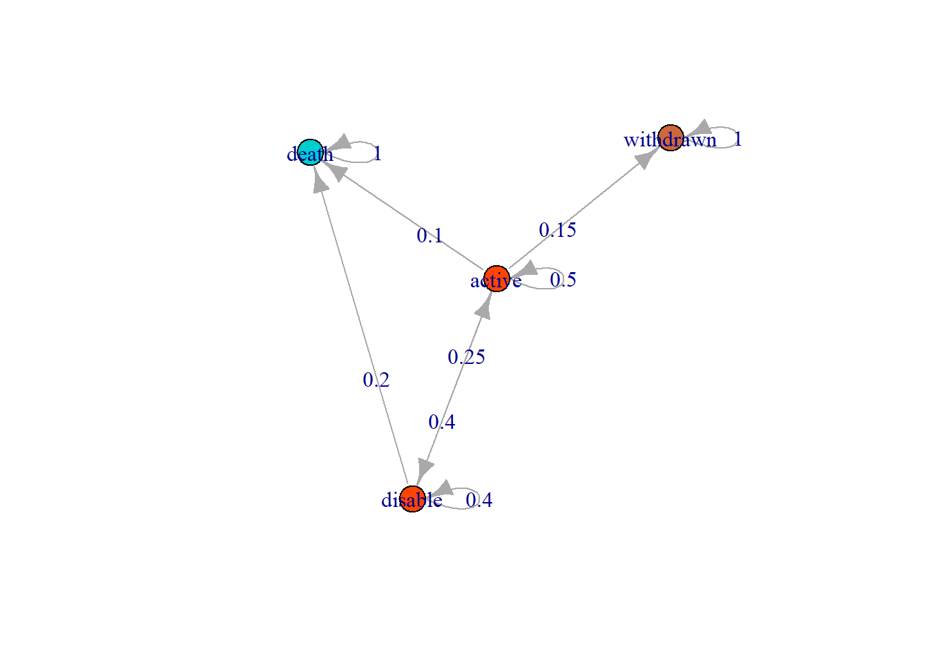
If the current state is withdrawn, the next state is certainly withdrawn as well since it has the transition probability of 1. The same thing happens when the current state is death. This state is called Absorbing States, because once the system entered this state, it cannot left. The system will loop and staty at the state. Once people withdrawn their insurance, they next state will stay withdrawn and cannot be active again. Once the insured is death, they cannot be active or alive again (hopefully).
markov_health <- new("markovchain", transitionMatrix = transition_matrix,
                    name = "Health Insurance",
                    states = c("active", "disable", "withdrawn", "death"))

markov_health
#> Health Insurance
#> A 4 - dimensional discrete Markov Chain defined by the following states:
#> active, disable, withdrawn, death
#> The transition matrix (by rows) is defined as follows:
#> active disable withdrawn death
#> active 0.5 0.25 0.15 0.1
#> disable 0.4 0.40 0.00 0.2
#> withdrawn 0.0 0.00 1.00 0.0
#> death 0.0 0.00 0.00 1.0To acquire the absorbing state of the Markov Chains, we simply use absorbingState() function.
absorbingStates(markov_health)#> [1] "withdrawn" "death"Based on the result, the absorbing state for Health Insurance is withdrawn and death.
Transient State and Recurrent State
A state is said to be a transient state if, upon entering this state, the process might never return to this state again.
transientStates(markov_health)#> [1] "active" "disable"State active and disable is transient because there is a non-zero probability that we will never return to this state.
Meanwhile, a state is said to be a recurrent state if, upon entering this state, the process definitely will return to this state again. Therefore, a state is recurrent if and only if it is not transient.
recurrentStates(markov_health)#> [1] "withdrawn" "death"State withdrawn and death is recurrent because there is no non-zero probability that we will never return to this state.
Text Generation
This part will illustrate how Markov Chain can be applied to make a text generator. There are some advantages of employing Markov Chains for text generation compared to other method:
- Simple and easy to implement
- Lower computation time
However, there is some disadvantages on using Markov Chains to build text generator:
- The generated text is as good as the input corpus (garbage in garbage out)
- Need to create multiple n-gram Markov Chains (high order model) to captue the context
Before we create a big and complex text generator using a corpus or collection of text data, first let’s create a simple one. I will use a single sentence and build a text generator based on words present on the sentence.
 {width = “40%”}
First, we prepare the sentence, a generic sentence that is used as a benchmark to test fonts: the quick brown fox jumps over the lazy dog. I will make it longer into the quick brown fox jumps over the lazy dog and the angry dog chase the fox. This single text will be splitted/tokenized without eliminating the word sequences.
# a single sentence
short_text <- c("the quick brown fox jumps over the lazy dog and the angry dog chase the fox")

# split the sentence into words
text_term <- strsplit(short_text, split = " ") %>% unlist()

short_text
#> [1] "the quick brown fox jumps over the lazy dog and the angry dog chase the fox"text_term#> [1] "the" "quick" "brown" "fox" "jumps" "over" "the" "lazy" "dog"
#> [10] "and" "the" "angry" "dog" "chase" "the" "fox"Now that we have the terms and it’s sequence, we can build a Markov Chains and visualize the networks.
fit_markov <- markovchainFit(text_term, method = "laplace")

set.seed(123)
plot(fit_markov$estimate)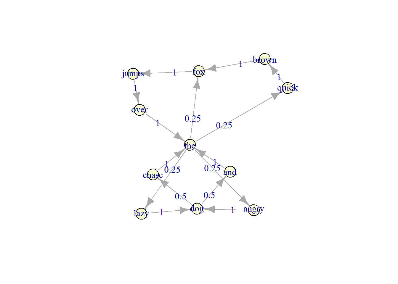
fit_markov$estimate#> Laplacian Smooth Fit
#> A 11 - dimensional discrete Markov Chain defined by the following states:
#> and, angry, brown, chase, dog, fox, jumps, lazy, over, quick, the
#> The transition matrix (by rows) is defined as follows:
#> and angry brown chase dog fox jumps lazy over quick the
#> and 0.0 0.00 0 0.0 0 0.00 0 0.00 0 0.00 1
#> angry 0.0 0.00 0 0.0 1 0.00 0 0.00 0 0.00 0
#> brown 0.0 0.00 0 0.0 0 1.00 0 0.00 0 0.00 0
#> chase 0.0 0.00 0 0.0 0 0.00 0 0.00 0 0.00 1
#> dog 0.5 0.00 0 0.5 0 0.00 0 0.00 0 0.00 0
#> fox 0.0 0.00 0 0.0 0 0.00 1 0.00 0 0.00 0
#> jumps 0.0 0.00 0 0.0 0 0.00 0 0.00 1 0.00 0
#> lazy 0.0 0.00 0 0.0 1 0.00 0 0.00 0 0.00 0
#> over 0.0 0.00 0 0.0 0 0.00 0 0.00 0 0.00 1
#> quick 0.0 0.00 1 0.0 0 0.00 0 0.00 0 0.00 0
#> the 0.0 0.25 0 0.0 0 0.25 0 0.25 0 0.25 0The subsequent words are generated based on the transition probability (the number on the graph). For example, if the current word is dog, the next word can be chase and word and, with equal probability of 0.5 to appear. If the current word is chase, the next word must be the because it has probability of 1 to appear afer word chase.
Now we can try to generate a text using the markov chain. Here, I only type word the and let the model finish the sentence. We will generate 5 different phrases.
# generate random sentence
for (i in 1:5) {

   set.seed(i)
   markovchainSequence(n = 7, # generate 7 next words
                       markovchain = fit_markov$estimate, # transition matrix
                       t0 = "the", include.t0 = T) %>%  # set the first word

   # joint words
   paste(collapse = " ") %>%
   paste0(".") %>%
   print()
}
#> [1] "the fox jumps over the angry dog chase."
#> [1] "the angry dog chase the quick brown fox."
#> [1] "the angry dog and the lazy dog and."
#> [1] "the lazy dog and the quick brown fox."
#> [1] "the angry dog chase the angry dog chase."Does the sentences make sense? Perhaps some of them does. The number of words generated also affect whether the sentence will make sense or not, such as the third sentence that end with and, making it an incomplete sentence, while the second and fourth sentence can be a complete sentence. We may want to cut the sentence at certain point to make it a better sentence.
Next, we can try to create more complex model using to create a sentences based on Sherlock Holmes novel.
Import Dataset
The data come from The Adventure of Sherlock Holmes by Sir Arthur Conan Doyles. We will directly import the text from the project gutenberg website. Since processing a lot of words/terms in NLP is requires a huge resource (both times and power), I will only use this single book instead of all of Sherlock Holmes novels.
library(gutenbergr)

sherlock <- gutenberg_download(1661)
head(sherlock, 30)
#> # A tibble: 30 x 2
#> gutenberg_id text
#> <int> <chr>
#> 1 1661 "THE ADVENTURES OF SHERLOCK HOLMES"
#> 2 1661 ""
#> 3 1661 "by"
#> 4 1661 ""
#> 5 1661 "SIR ARTHUR CONAN DOYLE"
#> 6 1661 ""
#> 7 1661 ""
#> 8 1661 ""
#> 9 1661 " I. A Scandal in Bohemia"
#> 10 1661 " II. The Red-headed League"
#> # ... with 20 more rowsText Cleansing
We need to cleanse the text and remove the chapter title and unnecessary element such as blank text.
# Get chapter title
chapter_title <- sherlock %>%
   filter(text != "") %>%
   slice(c(4:15)) %>%
   pull(text) %>%
   tolower() %>%
   str_trim()

# text cleansing
sherlock_clean <- sherlock %>%
   mutate(text  = tolower(text)) %>%
   filter( str_detect(text, paste(chapter_title, collapse = "|")) == F,
           text != "") %>%
   slice(-c(1:4)) %>%
   mutate(text = text %>%
             str_replace(pattern = "--", " ") %>%
             # remove punctuation selain tanda titik, koma sama seru
             str_remove_all(pattern = "(?![.,!])[[:punct:]]") %>%
             str_remove_all(pattern = "[0-9]") %>% # remove numeric
             replace_contraction() %>% # I'll menjadi I will
             replace_white() %>% # remove double white space
             str_replace_all("mrs[.]", "mistress") %>%
             str_replace_all("mr[.]", "mister") %>%
             str_replace_all(pattern = "[.]", replacement = " .") %>%
             str_replace_all(pattern = "[!]", replacement = " !") %>%
             str_replace_all(pattern = "[,]", replacement = " ,"))

head(sherlock_clean, 10)
#> # A tibble: 10 x 2
#> gutenberg_id text
#> <int> <chr>
#> 1 1661 to sherlock holmes she is always the woman . i have seldom heard
#> 2 1661 him mention her under any other name . in his eyes she eclipses
#> 3 1661 and predominates the whole of her sex . it was not that he felt
#> 4 1661 any emotion akin to love for irene adler . all emotions , and t~
#> 5 1661 one particularly , were abhorrent to his cold , precise but
#> 6 1661 admirably balanced mind . he was , i take it , the most perfect
#> 7 1661 reasoning and observing machine that the world has seen , but a~
#> 8 1661 lover he would have placed himself in a false position . he nev~
#> 9 1661 spoke of the softer passions , save with a gibe and a sneer . t~
#> 10 1661 were admirable things for the observer excellent for drawing theEach row represent a single line in the book. To get better result, first we need to make a compile all row into a single vector.
text_sherlock <- sherlock_clean %>%
   pull(text) %>%
   strsplit(" ") %>%
   unlist()

text_sherlock %>% head(30)
#> [1] "to" "sherlock" "holmes" "she" "is"
#> [6] "always" "the" "woman" "." "i"
#> [11] "have" "seldom" "heard" "him" "mention"
#> [16] "her" "under" "any" "other" "name"
#> [21] "." "in" "his" "eyes" "she"
#> [26] "eclipses" "and" "predominates" "the" "whole"n_distinct(text_sherlock)#> [1] 8198Model Fitting
Now we will fit the data into Markov Chains.
fit_markov <- markovchainFit(text_sherlock)Let’s try to generate some sentences based on the Markov Chains. We will generate the next 6 words.
for (i in 1:10) {

   set.seed(i)

   markovchainSequence(n = 10,
                       markovchain = fit_markov$estimate,
                       t0 = "the", include.t0 = T) %>%

   # joint words
   paste(collapse = " ") %>%

   # create proper sentence form
   str_replace_all(pattern = " ,", replacement = ",") %>%
   str_replace_all(pattern = " [.]", replacement = ".") %>%
   str_replace_all(pattern = " [!]", replacement = "!") %>%

   str_to_sentence() %>%

   print()
}
#> [1] "The windows of some mystery. ill swing for this is"
#> [1] "The only reached her own seal and the stripped body of"
#> [1] "The name which had, in that i should think of"
#> [1] "The river, but he shot out a gipsy had been"
#> [1] "The king stared from his head gravely. perhaps except when"
#> [1] "The injuries which was that for robbery at our friends and"
#> [1] "The pink flush upon the ground to a wash, which"
#> [1] "The mystery. to open the girl, brilliant beam of"
#> [1] "The one of the street, and in his costume is"
#> [1] "The subject. there he was no doubt that, he"If you want to make the model as a predictive text, you can create a function that will return a set of words with the highest probability for the next step.
predictive_text <- function(text, num_word){
   text <- strsplit(text, " ") %>% unlist() %>% tail(1)

   # exclude punctuation
   punctuation <- which(fit_markov$estimate[ tolower(text), ] %>% names() %>% str_detect("[:punct:]"))

   suggest <- fit_markov$estimate[ tolower(text), -punctuation] %>%
   sort(decreasing = T) %>%
   head(num_word)

   suggest <- suggest[suggest > 0] %>%
   names()

   return(suggest)
}

predictive_text("i am", 10)
#> [1] "sure" "not" "afraid" "a" "so" "sorry" "very" "glad"
#> [9] "in" "all"Since we only use a token (1-gram), the Markov Chains will only consider the last word and see no context or sequence of words in the sentence.
predictive_text("i wish she", 10)#> [1] "had" "was" "is" "has" "would" "cried" "could" "said" "will"
#> [10] "saw"Text Generation with N-gram
The previous section tell us how to create a Markov Chains text generator with a single term (1-gram) token. Can we create a Markov Chain using bigram (2-grams) or trigram (3-grams)?
The answer is yes. We just need to adjust the input to be an n-grams instead of a single term.
Bigram Predictive Text
Bigram predictive text will use two consecutive words/terms in order to predict the next word, instead of only using the last word. The transition matrix will consists of the transition probability between bigram.
bigram_sherlock <- sherlock_clean %>%
   head(2000) %>%
   unnest_tokens(bigram, text, token = "ngrams", n = 2) %>%
   pull(bigram)

bigram_sherlock %>% head(10)
#> [1] "to sherlock" "sherlock holmes" "holmes she" "she is"
#> [5] "is always" "always the" "the woman" "woman i"
#> [9] "i have" "have seldom"We will fit the vector into the Markov Chains. However, since the huge amount of bigram text and my hardware limitation, I can only afford to fit the first 2000 observations of the text. This will affect the transition matrix, but since we (more precisely me) don’t have a lot of options, we will proceed to the next step. The fitting process take a lot of time to process and I have saved the .Rds file for you to access.
markov_bigram <- markovchainFit(bigram_sherlock)markov_bigram <- read_rds("data_input/bigram_sherlock.Rds")We will create a predictive text function using the Bigram Markov Chains. Let’s say if I insert i will, what will be the top 5 next words.
predictive_text <- function(text, num_word){

   suggest <- markov_bigram$estimate[ tolower(text), ] %>%
   sort(decreasing = T) %>%
   head(num_word)

   suggest <- suggest[ suggest > 0] %>%
   names() %>%
   str_extract(pattern = "\\s(.*)") %>%
   str_remove("[ ]")

   return(suggest)
}

predictive_text("i will", 5)
#> [1] "be" "follow" "get" "make" "not"We can also create a random text generator using the bigram to create sentences.
library(stringi)

for (i in 1:10) {

   set.seed(i)

   markovchainSequence(n = 10,
                       markovchain = markov_bigram$estimate,
                       t0 = "i was", include.t0 = T) %>%
   stri_extract_last_words() %>%

   # joint words
   c("i", .) %>%
   paste(collapse = " ") %>%

   # create proper sentence form
   str_replace_all(pattern = " ,", replacement = ",") %>%
   str_replace_all(pattern = " [.]", replacement = ".") %>%
   str_replace_all(pattern = " [!]", replacement = "!") %>%

   str_to_sentence() %>%

   print()
}
#> [1] "I was certain that it means i have often thought the reaction"
#> [1] "I was aware that i had my note he asked does it"
#> [1] "I was always well dressed and ill swing for it made me"
#> [1] "I was still raised to it i could fathom then they carried"
#> [1] "I was aware that i have heard some vague account of you"
#> [1] "I was conspiring or the bullion might be removed saturday would suit"
#> [1] "I was about to be a little square of cardboard hammered on"
#> [1] "I was a royal duke and he said that she had probably"
#> [1] "I was aware of it in twenty minutes it was close upon"
#> [1] "I was compelled to open and an elderly woman stood upon the"Trigram Predictive Text
We will also create a Markov Chains for Trigram to get the context up to 3 previous words. However, since the huge amount of trigram text and my hardware limitation, I can only afford to fit the first 2000 observations of the text.
trigram_sherlock <- sherlock_clean %>%
   head(2000) %>%
   unnest_tokens(bigram, text, token = "ngrams", n = 3) %>%
   pull(bigram)

trigram_sherlock %>% head(10)
#> [1] "to sherlock holmes" "sherlock holmes she" "holmes she is"
#> [4] "she is always" "is always the" "always the woman"
#> [7] "the woman i" "woman i have" "i have seldom"
#> [10] "have seldom heard"Fit the data into Markov Chains. The fitting process take so much time so I save the .Rds file for you to access.
markov_trigram <- markovchainFit(trigram_sherlock)markov_trigram <- read_rds("data_input/trigram_sherlock.Rds")Create the predictive function.
predictive_text <- function(text, num_word){

   suggest <- markov_trigram$estimate[ tolower(text), ] %>%
   sort(decreasing = T) %>%
   head(num_word)

   suggest <- suggest[ suggest > 0 ] %>%
   names() %>%
   str_extract(pattern = "\\s(.*)") %>%
   str_remove("[ ]") %>%
   str_extract(pattern = "\\s(.*)") %>%
   str_remove("[ ]")

   return(suggest)
}

predictive_text("i wish you", 5)
#> [1] "would"Combine 3 Markov Chains
We can combine all Markov N-grams into a single function. The benefit is that it will look for context in trigram and bigram. If the input text has 3 or more words, it will look at the last 3 words on the phrase. If the words are not identified from the trigram Markov Chains or if the phrase has only 2 words, it will look at the bigram Markov Chains instead. Finally, if the two Markov Chains failed to find the result from their respective transition matrix, we will look at the 1-gram Markov Chains to predict the next word. I have compiled it in an R script.
- Mencari kemungkinan atau state di 3-gram
- Kalau tidak ada, cari di 2-gram
- Kalau tidak ada, cari di 1-gram
source("markov_predictive.R")

predictive_text("i love", num_word = 5)
#> [1] "own" "friend" "dear" "companion" "wife"Business Use Case
There are many application of Markov Chains in various field of industries other than for text generation. On this section, I will illustrate some use cases of Markov Chains in health insurance and manufacturing machine maintenance.
You may skip the next sections if you only wish to learn how to create a text generator.
Machine Maintenance
This problem is derived from Hillier and Lieberman11. A manufacturer has one key machine at the core of one of its production processes. Because of heavy use, the machine deteriorates rapidly in both quality and output. Therefore, at the end of each week, a thorough inspection is done that results in classifying the condition of the machine into one of four possible states:
- 1: Good - No apparent problem
- 2: Operable with minor deterioration
- 3: Operable with major deterioration
- 4: Inoperable due to bad quality
The transition matrix for this problem is as follows.
transition_matrix <- matrix(c(0, 7/8, 1/16, 1/16,
                              0, 3/4, 1/8, 1/8,
                              0, 0, 1/2, 1/2,
                              1, 0, 0, 0),
                            byrow = TRUE, nrow = 4)

transition_matrix
#> [,1] [,2] [,3] [,4]
#> [1,] 0 0.875 0.0625 0.0625
#> [2,] 0 0.750 0.1250 0.1250
#> [3,] 0 0.000 0.5000 0.5000
#> [4,] 1 0.000 0.0000 0.0000Based on the transition matrix, we can see that an inoperable machine will go back to the state of Good as new. This is because the company cannot let the machine to stay broken since the production target must be met. The machine would be repaired or replaced. The replacement process takes 1 week to complete so that production is lost for this period. The cost of the lost production (lost profit) is USD 2,000, and the cost of replacing the machine is USD 4,000; so the total cost incurred whenever the current machine enters state 4 is USD 6,000. Even before the machine reaches state 3, costs may be incurred from the production of defective items. When the machine is in minor deteroriation (state 2), the expected costs per week is USD 1,000 while if the machine is in a major deteroriation (state 3), the expected cost per week is USD 3,000. Another cost that can be incurred is when we do an overhaul toward the machine, which incurr USD 2000 for maintenance while also making us lost USD 2000 of profit.
Below is the complete list of the cost and when the cost can be incurred:
cost_df <- data.frame(policy = c("do nothing", "do nothing", "do nothing", "overhaul", "replace"),
           state = c(1, 2, 3, 4, "2, 3, 4"),
           cost_due_to_defect = c(0, 1000, 3000, 0, 0),
           maintenance_cost = c(0, 0, 0, 2000, 4000),
           profit_lost = c(0, 0, 0, 2000, 2000),
           total_cost = c(0, 1000, 3000, 4000, 6000)
           )

cost_df
#> policy state cost_due_to_defect maintenance_cost profit_lost total_cost
#> 1 do nothing 1 0 0 0 0
#> 2 do nothing 2 1000 0 0 1000
#> 3 do nothing 3 3000 0 0 3000
#> 4 overhaul 4 0 2000 2000 4000
#> 5 replace 2, 3, 4 0 4000 2000 6000What is the optimal maintenance policy? Should we do nothing at all? Or do we need to overhaul everytime the machine go to major deteroriation (state 3)? Do we need to replace the machine every time it deviate from state 1? We will discuss it one at a time.
First, from the transition matrix, we will create a markovchain object.
markov_model <- new("markovchain", transitionMatrix = transition_matrix,
                    name = "Machine Opeation", states = c("Good", "Minor", "Major", "Inoperable"))

set.seed(123)
plot(markov_model)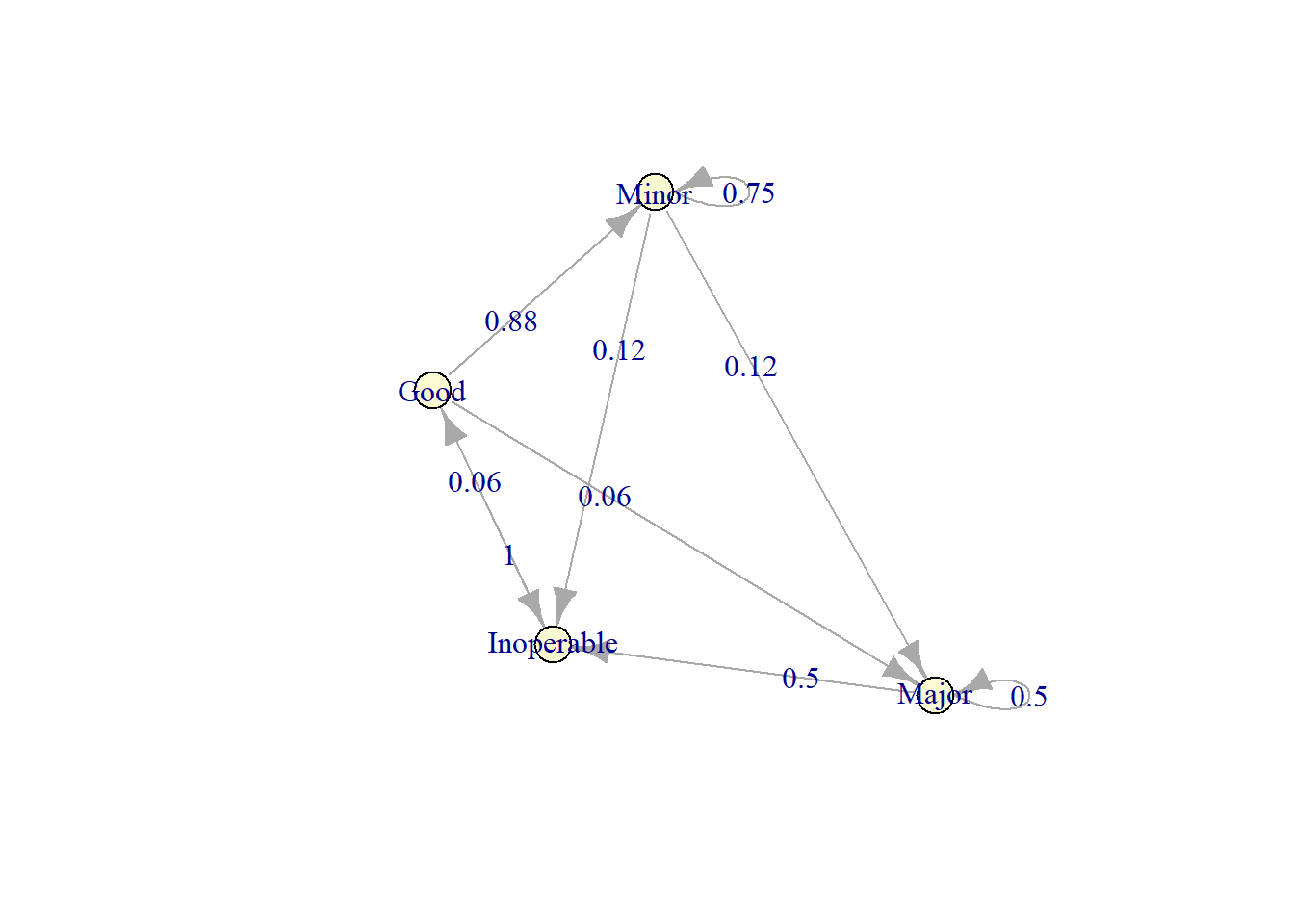
First Policy
First we will employ the policy to replace the machine eveytime it reach the inoperable condition (state 1).
To evaluate this maintenance policy, we should consider both the immediate costs incurred over the coming week (just described) and the subsequent costs that result from having the system evolve in this way. A widely used measure of performance for Markov chains is the (long-run) expected average cost per unit time. To calculate this measure, we first derive the steady-state probabilities. If you remember, steady-state means that regardless of the previous state, the probability for the next is all the same.
steadyStates(markov_model)#> Good Minor Major Inoperable
#> [1,] 0.1538462 0.5384615 0.1538462 0.1538462Hence, the (long-run) expected average cost per week for this maintenance policy is:
\[0\ \pi_1 + 1000\ \pi_2\ +\ 3000\ \pi_3\ +\ 6000\ \pi_4\]
cost <- c(0, 1000, 3000, 6000)

policy_1 <- (steadyStates(markov_model) * cost) %>% sum()
policy_1
#> [1] 1923.077If we replace the machine eveytime it reach the inoperable condition (state 4), the expected cost is USD 1923.08.
Second Policy
The second policy is to replace the machine when it is inoperable (state 4) and overhaul it when it get to major deteroriation (state 3). Since overhauling can make our machine condition to be better, the transition matrix is changed from the previous one. Everytime the machine get overhauled, it would go from major deteroriation to minor deteroriation.
transition_matrix <- matrix(c(0, 7/8, 1/16, 1/16,
                              0, 3/4, 1/8, 1/8,
                              0, 1, 0, 0,
                              1, 0, 0, 0),
                            byrow = TRUE, nrow = 4)

markov_model <- new("markovchain", transitionMatrix = transition_matrix,
                    name = "Machine Opeation", states = c("Good", "Minor", "Major", "Inoperable"))

set.seed(123)
plot(markov_model)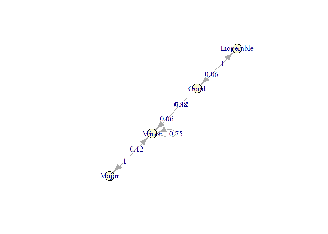
By employing overhaul with cost of USD 4000,the cost for state 3 goes from mere USD 3000 (cost due to defect) to USD 4000.
The expected average cost is as follows.
cost <- c(0, 1000, 4000, 6000)

policy_2 <- (steadyStates(markov_model) * cost) %>% sum()
policy_2
#> [1] 1666.667Third Policy
The third policy is to replace the machine every time it goes to state 3 and state 4. The transition matrix is once again change, because by replacing the machine, it will go from state 3 directly toward state 1 (Good) instead of going to state 2 (minor deteroriation).
transition_matrix <- matrix(c(0, 7/8, 1/16, 1/16,
                              0, 3/4, 1/8, 1/8,
                              1, 0, 0, 0,
                              1, 0, 0, 0),
                            byrow = TRUE, nrow = 4)

markov_model <- new("markovchain", transitionMatrix = transition_matrix,
                    name = "Machine Opeation", states = c("Good", "Minor", "Major", "Inoperable"))

set.seed(123)
plot(markov_model)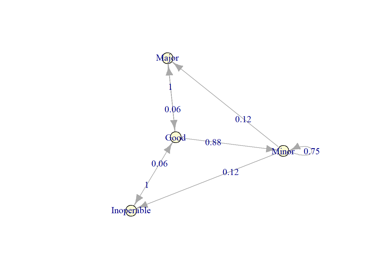
The expected average cost is as follows.
cost <- c(0, 1000, 6000, 6000)

policy_3 <- (steadyStates(markov_model) * cost) %>% sum()
policy_3
#> [1] 1727.273We recap the cost associated with each policy.
data.frame(policy = c("Only replace machine when inoperable", "Replace and overhaul", "Replace when major deteroriation and inoperable"),
           `expected cost` = c(policy_1, policy_2, policy_3))
#> policy expected.cost
#> 1 Only replace machine when inoperable 1923.077
#> 2 Replace and overhaul 1666.667
#> 3 Replace when major deteroriation and inoperable 1727.273Based on the expected average cost, we can see that by combining machine replacement and overhaul, we can expect the minimum cost. Thus, we should employ this policy. There are a lot of other application of Markov Chains in manufacturing, such as in inventory management, quality control, even in customer management.
Health Insurance
Actuaries quantify the risk inherent in insurance contracts, evaluating the premium of insurance contract to be sold (therefore covering future risk) and evaluating the actuarial reserves of existing portfolios (the liabilities in terms of benefits or claims payments due to policyholder arising from previously sold contracts). The example comes from Deshmukh[^12].
An insurer issues a special 3-year insurance contract to a person when the transitions among four states, 1: active, 2: disabled, 3: withdrawn, and 4: dead. The death benefit is 1000, payable at the end of the year of death. A death benefit is a payout to the beneficiary of a life insurance policy, annuity, or pension when the insured or annuitant dies. Suppose that the insured is active at the issue of policy. Insureds do not pay annual premiums when they are disabled. Suppose that the interest rate is 5 % per annum. Calculate the benefit reserve at the beginning of year 2 and 3.
benefit <- c(0, 0, 500, 1000)

transition_matrix <- matrix(c(0.5, .25, .15, .1,
                              0.4, 0.4, 0.0, 0.2,
                              0, 0, 1, 0,
                              0, 0, 0, 1),
                            byrow = TRUE, nrow = 4)

markov_model <- new("markovchain", transitionMatrix = transition_matrix,
                    name = "Health Insurance", states = c("active", "disable", "withdrawn", "death"))

set.seed(1000)
plot(markov_model)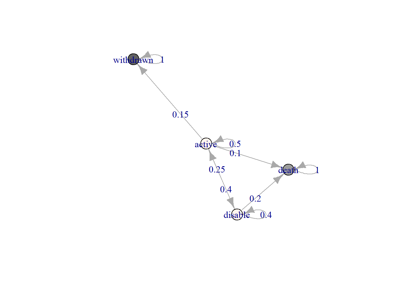
The policyholders is active at \(T_0\). Therefore the expected states at \(T_1, T_2, T_3\) are calculated in the following.
T0 <- c(1,0,0,0)
T1 <- T0 * markov_model
T2 <- T1 * markov_model
T3 <- T2 * markov_model

paste(c("Year 0:", T0), collapse = " ")
#> [1] "Year 0: 1 0 0 0"paste(c("Year 1:", T1), collapse = " ")#> [1] "Year 1: 0.5 0.25 0.15 0.1"paste(c("Year 2:", T2), collapse = " ")#> [1] "Year 2: 0.35 0.225 0.225 0.2"paste(c("Year 3:", T3), collapse = " ")#> [1] "Year 3: 0.265 0.1775 0.2775 0.28"The present value of future benefit (PVFB) at T0 is given by:
PVFB <- T0 %*% benefit * 1.05 ^ -0 +
   T1 %*% benefit * 1.05 ^ -1 +
   T2 %*% benefit * 1.05 ^ -2 +
   T3 %*% benefit * 1.05 ^ -3

PVFB
#> [,1]
#> [1,] 811.8454The yearly premium payable whether the insured is alive is as follows.
P <- PVFB / (T0[1] * 1.05 ^- 0 + T1[1] * 1.05 ^ -1 + T2[1] * 1.05 ^ -2)The reserve at the beginning of the second year, in the case of the insured being alive, is as follows.
PVFB <- T2 %*% benefit * 1.05 ^ -1 + T3 %*% benefit * 1.05 ^ -2
PVFP <- P*(T1[1] * 1.05 ^ -0 + T2[1] * 1.05 ^ -1)

PVFB - PVFP
#> [,1]
#> [1,] 300.2528Conclusion
Markov Chains is a simple yet effective method to create a predictive text model. It model the transition probability between states, where in NLP each state is represented by terms/words. However, since it rely only on the probability of transition between words, the text generator still feel like a random mess when creating a sentence and has no context. Regardless, Markov Chains can be applied as a predictive text using combination of 1-gram, 2-grams, and 3-grams text.
The main challenge on employing an NLP model is the hardware and computational power. Perhaps in the future we would like to consider to make a text generator with Deep Learning model and compare the performance with the current Markov Chains model. Beside of its application in NLP, Markov Chains is also proven to be useful in many other fields such as maintenance and healh insurance.


 More details
 More details
Share this post
Twitter
Facebook
LinkedIn