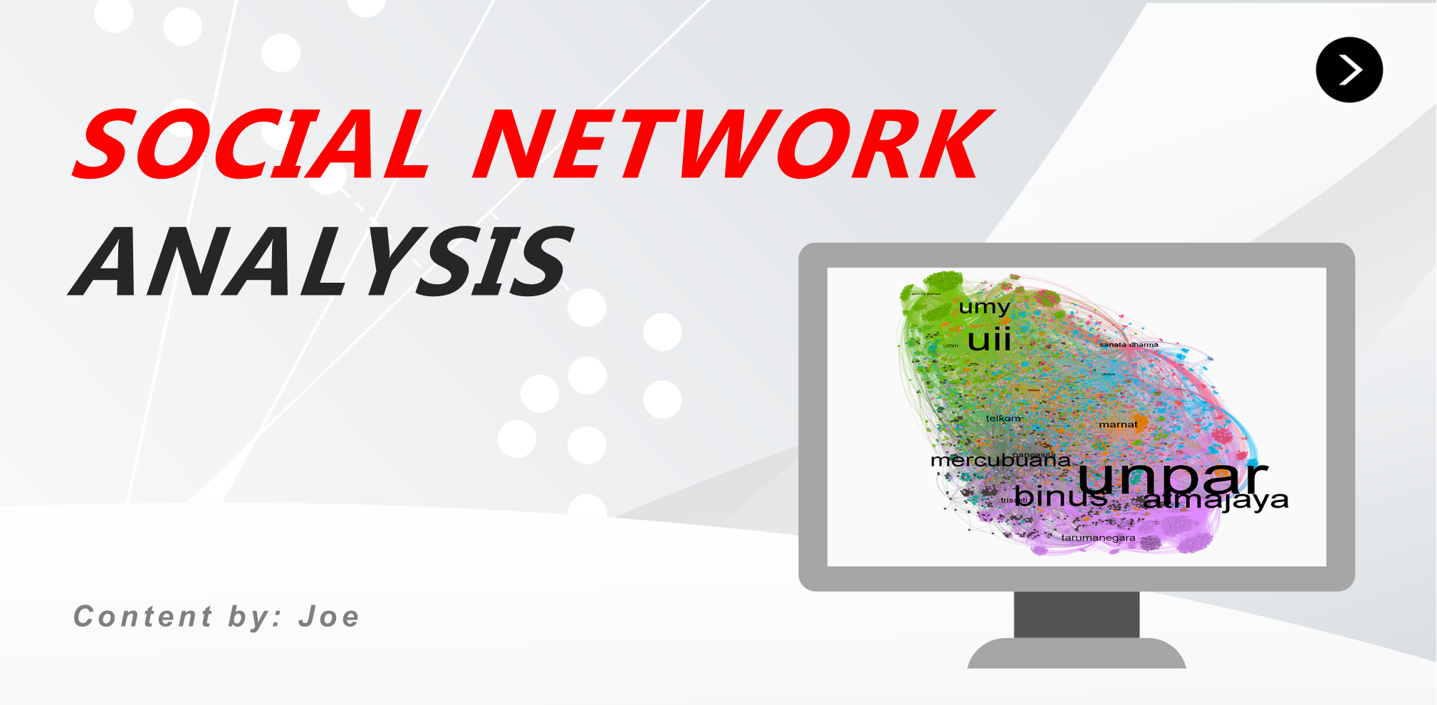
In this article, we will learn about Social Network Analysis using tidygraph (including igraph and ggraph). We’ll not only learn about the visualizing stuff but also the metrics. We’ll analyze Twitter network as our study case using rtweet package. In this article, I hope we will be able to do:
- Analyze Ego Network from specific account/user
- Analyze Information Activity Network from something that goes viral
Background
Introduction
What is Social Network Analysis (SNA)
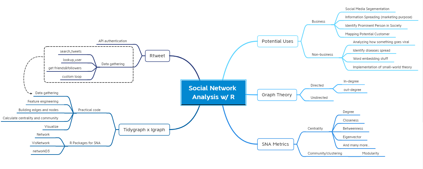
A social network is a structure composed of a set of actors, some of which are connected by a set of one or more relations. Social network analysis work at describing underlying patterns of social structure, explaining the impact of such patterns in behavior and attitudes. Social network analysis has 4 main types of network metrics, namely:
- Network Models: Describe how to model the relationship between users
- Key Players: To identify the most influential users in the network based on a different context
- Tie Strength: To measure the strength of a user’s relationship
- Network Cohesion: To measure how cohesive entities in the networks towards network behavior.
So what? Why do we need them?
Humans are social beings. Even when you sleep, you’re still connected to everyone in the world by your smartphone. Your smartphone keeps sending and receive information like weather information, incoming whatsapp messages, late-night One Piece update, and social media notification from your favorite bias. We’re always connected and there’s network everywhere. Somehow, some smart dudes behind the famous Small World Theory found something from the network that quite exciting.
Did you know you only seperates by six steps from your favorite person in the world? We are able to quantify the what-so-called network and can be implemented in many fields. In this study, we’ll only focus on identify network metrics with key player as the expected output (see the 4 main types of network metrics above). Here’s some implementation of SNA to enlight your knowledge about SNA a bit:
- Business:
- Non-business:
- Analyzing how something goes viral in social media
- Identify diseases spread
- Word embedding stuff
- Implementation of small-world theory and Six degree separation of Kevin Bacon
- Analyzing how something goes viral in social media
Libraries
Let’s install required library for this study.
# for data wrangling. very helpfull for preparing nodes and edges data
library(tidyverse)
library(lubridate)

# for building network and visualization
library(tidygraph)
library(graphlayouts)
# already included in tidygraph but just fyi
library(igraph)
library(ggraph)

# for crawling Twitter data
library(rtweet)
Let’s Begin !
Prerequisites
We’ll crawl Twitter data using Twitter’s rest API. Thus, we need authentication to use the API. To access the API, you will need to create a Twitter Developer Account here: https://developer.twitter.com/en (make sure you already have Twitter account). Creating a Twitter developer account is simple and tends to be fast but it depend on how you describe what you will do with the API.
Good news! recent update of rtweet allows you to interact with Twitter API without creatin your own Twitter developer account. But it’s better if you have one because it gives you more stability and permissions. If you need further explanation, you can head over rtweet’s official website here.
apikey <- "A5csjkdrS2xxxxxxxxxxx"
apisecret <- "rNXrBbaRFVRmuHgEM5AMpdxxxxxxxxxxxxxxxxxxxxxxx"
acctoken <- "1149867938477797376-xB3rmjqxxxxxxxxxxxxxxxxxxx"
tokensecret <- "Dyf3VncHDtJZ8FhtnQ5Gxxxxxxxxxxxxxxxxxxxxxx"

token <- create_token(app = "Automated Twitter SNA",
                      consumer_key = apikey,
                      consumer_secret = apisecret,
                      access_token = acctoken,
                      access_secret = tokensecret)
# Note: Only run one this code if you cant crawl the data without using any access token
mytoken_1 <- readRDS("data_input/SNA/token_1.rds")
#mytoken_2 <- readRDS("data_input/token_2.rds")
# check if the token is active
get_token()#> <Token>
#> <oauth_endpoint>
#> request: https://api.twitter.com/oauth/request_token
#> authorize: https://api.twitter.com/oauth/authenticate
#> access: https://api.twitter.com/oauth/access_token
#> <oauth_app> Automated Twitter SNA
#> key: A5csjkdrS24vJ5ktiKYtgasFY
#> secret: <hidden>
#> <credentials> oauth_token, oauth_token_secret
#> ---Graph Theory
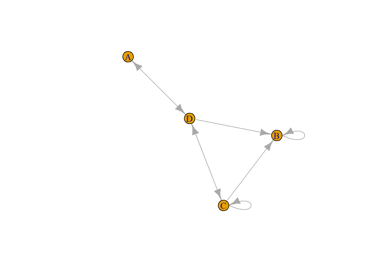
In mathematics, graph theory is the study of graphs, which are mathematical structures used to model pairwise relations between objects. A graph in this context is made up of vertices (also called nodes or points) which are connected by edges (also called links or lines). In general, A connection between nodes are separated by 2 types: Directed and Undirected.
Directed is a relationship between nodes that the edges have a direction (The edges have orientations). You will recognize it as edges that have an arrow in it. Directed network also separated into 2 types based on its direction, namely: in-degree and out-degree. In-degree represents the number of edges incoming to a vertex/node. In below directed graph, In-degree of A is 1 and degree of D is 2. Out-degree represents the number of edges outgoing from a vertex. In below directed graph, out-degree of A is 1 and out-degree of C is 3.
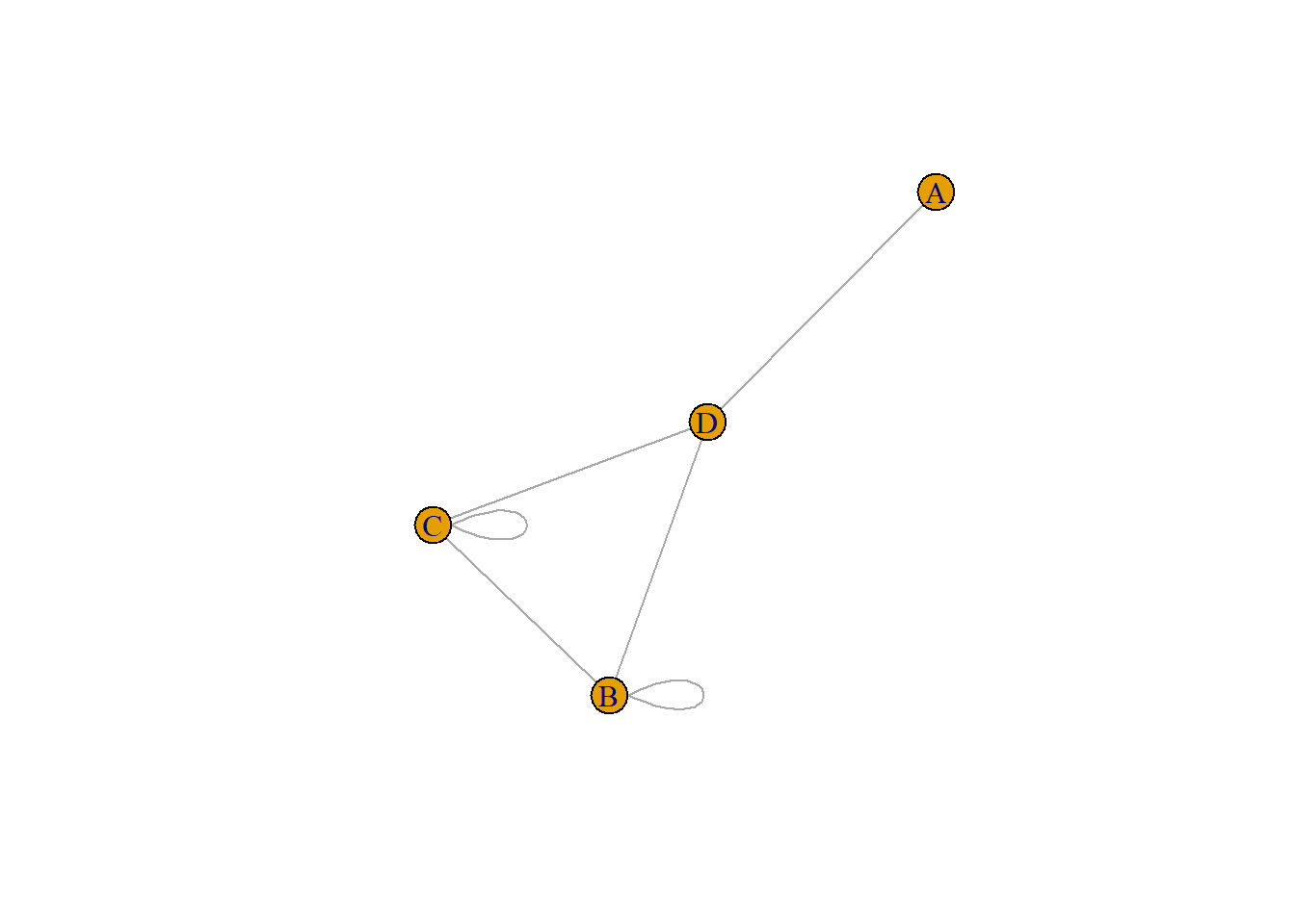
Undirected indicates a two-way relationship, the edges are unidirectional, with no direction associated with them. Hence, the graph can be traversed in either direction. The absence of an arrow tells us that the graph is undirected.
Case 1: TeamAlgoritma Ego Network
Ego network is a concept indicates the amount of all the nodes to which an ego/node is directly connected and includes all of the ties among nodes in a network. You take any random username/company/person you want to analyze, gather all their neighborhood, and analyze it. sometimes you’ll find interesting patterns like this person has a lot of different communities and none of them are look-alike, or you can also found a person who can spread information most widely around your target-person network.
Case objectives:
- Analyze Ego Network from @TeamAlgoritma Twitter account
+ Visualize top cluster from TeamAlgoritma mutual account
+ find out which account has the potential to spread information widely
+ Calculate the metrics, and find out who is the key player in TeamAlgoritma network
Here’s the step to do this case:
1. Gather TeamAlgoritma detail Twitter data
2. Gather all TeamAlgoritma followers
3. From the follower, filter to active account only and gather their follower and following
4. Create Mutual data from following and follower data
5. Build communities, Calculate SNA metrics, and identify which user is important
6. Visualize the ego network

Gather @TeamAlgoritma data
algo <- lookup_users("teamalgoritma")Gather TeamAlgoritma followers
# get teamalgoritma followers
folower <- get_followers("teamalgoritma",n = algo$followers_count,retryonratelimit = T)

# get the detail from algoritma follower lists
detail_folower <- lookup_users(folower$user_id)
detail_folower <- data.frame(lapply(detail_folower,as.character),stringsAsFactors = F)

detail_folower %>%
  arrange(-as.numeric(followers_count)) %>%
  select(screen_name,followers_count, friends_count, favourites_count) %>%
  head()
#> screen_name followers_count friends_count favourites_count
#> 1 btekno 331624 326 49
#> 2 machinelearnflx 93630 35370 160
#> 3 DD_FaFa_ 23531 16268 51250
#> 4 NgeeAnnNP 12198 186 9910
#> 5 TheMLHub 10454 9369 859
#> 6 CintaNegeri_ID 9116 8755 2975TeamAlgoritma Twitter account has 524 followers (on 2 February 2021). We need to gather all of their follower and following but Twitter rest API has (kinda stingy) limitation.
rate_limit()#> # A tibble: 217 x 7
#> query limit remaining reset reset_at timestamp app
#> <chr> <int> <int> <drtn> <dttm> <dttm> <chr>
#> 1 lists/~ 15 15 15.00~ 2021-03-16 16:38:57 2021-03-16 16:23:57 Autom~
#> 2 lists/~ 75 75 15.00~ 2021-03-16 16:38:57 2021-03-16 16:23:57 Autom~
#> 3 lists/~ 15 15 15.00~ 2021-03-16 16:38:57 2021-03-16 16:23:57 Autom~
#> 4 lists/~ 900 900 15.00~ 2021-03-16 16:38:57 2021-03-16 16:23:57 Autom~
#> 5 lists/~ 15 15 15.00~ 2021-03-16 16:38:57 2021-03-16 16:23:57 Autom~
#> 6 lists/~ 75 75 15.00~ 2021-03-16 16:38:57 2021-03-16 16:23:57 Autom~
#> 7 lists/~ 15 15 15.00~ 2021-03-16 16:38:57 2021-03-16 16:23:57 Autom~
#> 8 lists/~ 180 180 15.00~ 2021-03-16 16:38:57 2021-03-16 16:23:57 Autom~
#> 9 lists/~ 15 15 15.00~ 2021-03-16 16:38:57 2021-03-16 16:23:57 Autom~
#> 10 lists/~ 900 900 15.00~ 2021-03-16 16:38:57 2021-03-16 16:23:57 Autom~
#> # ... with 207 more rowsWe can only gather 15 users (both following and follower) and 5k retrieved for every 15 minutes, so you can imagine if we want to retrieve thousand of them.. In order to minimize the time consumption, we need to filter the users to active users only. The criteria of ‘active users’ depend on your data. You need to lookup which kind of users your follower is and build your own criteria. In this case, the top 8 of Algoritma’s followers is a media account. Accounts like ‘btekno’ and ‘machinelearnflx’ only repost link to their own media and never retweet other account tweets. So if our goal is to map the potential information spreading around TeamAlgoritma ego network, we need to exclude them for that reason.
After a long inspection, i propose several criteria for filtering active account: Followers_count > 100 and < 6000, following_count > 75, favourites_count > 10, and create a new tweet at least 2 months ago. I also want to exclude protected accounts because we actually can’t do anything about it, we can’t gather their following and followers.
active_fol <- detail_folower %>%
  select(user_id,screen_name,created_at,followers_count,friends_count,favourites_count) %>%
  mutate(created_at = ymd_hms(created_at),
         followers_count = as.numeric(followers_count),
         friends_count = as.numeric(friends_count),
         favourites_count = as.numeric(favourites_count)) %>%
  filter((followers_count > 100 & followers_count < 6000), friends_count > 75, favourites_count > 10,
         created_at > "2020-03-15") %>%
  arrange(-followers_count)
# TeamAlgoritma followers is always changing. we will use data i gathered at 5 March 2021
active_fol <- read.csv("data_input/SNA/active_fol_new.csv")Gather TeamAlgoritma follower’s follower
I build a loop function to gather followers from a list. Actually, we can gather the follower with this simple code
get_followers(active_fol$screen_name, n = "all",
              retryonratelimit = T)
But we want to minimize the total user we want to retrieve (n parameter). i build a simple function to retrieve half of the followers if they have more than 1500 followers, and 75% followers if they have less than 1500
flt_n <- function(x){
  if(x > 1500){
    x*0.5
  }else{x*0.75}
}
We also want to avoid SSL/TLS bug while we gather the followers. Sometimes when you reach the rate limit, the loop tends to crash and stop running. To avoid that, i order the loop to sleep every 5 gathered account (it doesn’t always solve the problem, but it way much better)
# Create empty list and name it after their screen name
foler <- vector(mode = 'list', length = length(active_fol$screen_name))
names(foler) <- active_fol$screen_name

#
for (i in 1:length(active_fol$screen_name)) {
  message("Getting followers for user #", i, "/", nrow(active_fol))
  foler[[i]] <- get_followers(active_fol$screen_name[i],
                                  n = round(flt_n(active_fol$followers_count[i])),
                                retryonratelimit = TRUE)

  if(i %% 5 == 0){
    message("sleep for 5 minutes")
    Sys.sleep(5*60)
    }
}
After gathering, bind the list to dataframe, convert the username to user_id by left_join from active_fol data, and build clean data frame without NA
# convert list to dataframe
folerx <- bind_rows(foler, .id = "screen_name")
active_fol_x <- active_fol %>% select(user_id,screen_name)

# left join to convert screen_name into its user id
foler_join <- left_join(folerx, active_fol_x, by="screen_name")

# subset to new dataframe with new column name and delete NA
algo_follower <- foler_join %>%
  select(user_id.x,screen_name) %>%
  setNames(c("follower","active_user")) %>%
  na.omit()
The loop need a looong time to be done. To speed up our progress, i already gather the followers and we’ll use it for analysis.
algo_follower_df <- read.csv("data_input/SNA/follower_algo_new.csv") Gather TeamAlgoritma follower’s following
Same as before, we build a loop function to gather the following. in rtweet package, following is also called as friend.
active_fol %>%
  arrange(-friends_count) %>%
  head(5)
#> user_id screen_name created_at followers_count
#> 1 447003337 YaromeerNedoman 2021-03-05 06:44:29 735
#> 2 1044599799058780160 SheShrugged 2021-03-04 14:38:16 414
#> 3 1451573756 ZanaPekmez 2021-02-25 22:05:20 1012
#> 4 5734262 alexajoyce 2021-03-04 20:13:41 2617
#> 5 2348301866 ameliazein 2021-03-05 05:53:43 1843
#> friends_count favourites_count
#> 1 5002 6530
#> 2 5001 6013
#> 3 4413 1546
#> 4 4065 578
#> 5 3991 5023As you can see, friends_count is way more higher than followers_count. Thus, we need to specify how many users we want to retrieve (n parameter). We want to minimize it, i change flt_n function to gather only 40% if they have more than 2k following, and 65% if less than 2k.
flt_n_2 <- function(x){
  if(x > 2000){
    x*0.4
  }else{x*0.65}
}
The loop is also a bit different. instead of list, we store the data to dataframe. get_friends() function gives 2 columns as their output; friend list and the query. we can easily just row bind them.
friend <- data.frame()

for (i in seq_along(active_fol$screen_name)) {
  message("Getting following for user #", i ,"/",nrow(active_fol))
  kk <- get_friends(active_fol$screen_name[i],
                        n = round(flt_n_2(active_fol$friends_count[i])),
                        retryonratelimit = TRUE)

  friend <- rbind(friend,kk)

  if(i %% 15 == 0){
    message("sleep for 15 minutes")
    Sys.sleep(15*60+1)
    }
}
all_friend <- friend %>% setNames(c("screen_name","user_id"))
all_friendx <- left_join(all_friend, active_fol_x, by="screen_name")
algo_friend <- all_friendx %>% select(user_id.x,screen_name) %>%
setNames(c("following","active_user"))This loop also takes a long time to run. Again, to speed up our progress, we will use the following data i already gathered.
algo_friend_df <- read.csv("data_input/SNA/following_algo_new.csv")We need to make sure all unique active user in algo_friend is available in algo_following and vice versa
algo_friend_df %>%
  filter(!active_user %in% algo_follower_df$active_user)
#> [1] following active_user
#> <0 rows> (or 0-length row.names)Create Mutual dataframe
Now we have both following and follower data. We need to build ‘mutual’ data to make sure the network is a strong two-side-connection network. Mutual is my terms of people who follow each other. we can found that by: split algo_friend data by every unique active_user, then we find every account in the following column that also appears in algo_follower$follower. The presence in both column indicates the user is following each other
# collect unique user_id in algo_friend df
un_active <- unique(algo_friend_df$active_user) %>%
  data.frame(stringsAsFactors = F) %>%
  setNames("active_user")

# create empty dataframe
algo_mutual <- data.frame()

# loop function to filter the df by selected unique user, then find user that presence
# in both algo_friend$following and algo_follower$follower column
# set column name, and store it to algo_mutual df

for (i in seq_along(un_active$active_user)){
  aa <- algo_friend_df %>%
    filter(active_user == un_active$active_user[i])
  bb <- aa %>% filter(aa$following %in% algo_follower_df$follower) %>%
    setNames(c("mutual","active_user"))

  algo_mutual <- rbind(algo_mutual,bb)
}head(algo_mutual)#> mutual active_user
#> 1 1078759789839011840 donkomo
#> 2 1294216335581310976 donkomo
#> 3 3739640056 donkomo
#> 4 955715941756583936 donkomo
#> 5 117810351 donkomo
#> 6 113292385 donkomoID represents user’s twitter id. We can get along with it but for me its not so interpretable. It will be better if we use their screen name. before that we need to lookup the profil detail using lookup_users()
detail_friend <- lookup_users(algo_mutual$mutual)detail_friend <- read.csv("data_input/SNA/detail_friend.csv")Then join the dataframe by user id and remove missing value
algo_mutual <- algo_mutual %>%
  left_join(detail_friend,by = c("mutual" = "user_id")) %>%
  na.omit()

head(algo_mutual)
#> mutual active_user screen_name
#> 1 1078759789839011840 donkomo alxmnt87
#> 3 3739640056 donkomo UvACORPNET
#> 5 117810351 donkomo WSWS_Updates
#> 6 113292385 donkomo airasia_indo
#> 7 1195245026831323136 donkomo AIswinarto
#> 8 33167774 donkomo benoistrousseauIt isn’t done yet. this is an ego network for TeamAlgoritma account, we want that account to appear on our screen. since TeamAlgoritma barely follows back its followers, it’s not a surprise if we can’t found it in mutual dataframe
# check if TeamAlgoritma is presence
algo_mutual %>%
  filter(mutual == "943736953274482688")
#> [1] mutual active_user screen_name
#> <0 rows> (or 0-length row.names)So we need to add them manually. we already have un_active dataframe contain unique value of active users. we can simply add extra column contain ’TeamAlgoritma" then bind them with algo_mutual df
un_active <- un_active %>%
  mutate(mutual = rep("TeamAlgoritma"))
# swap column oreder
un_active <- un_active[,c(2,1)]
un_active <- un_active %>%
  setNames(c("active_user","screen_name"))

# rbind to algo_mutual df
algo_mutual <- rbind(algo_mutual %>% select(-mutual),un_active)

head(algo_mutual)
#> active_user screen_name
#> 1 donkomo alxmnt87
#> 3 donkomo UvACORPNET
#> 5 donkomo WSWS_Updates
#> 6 donkomo airasia_indo
#> 7 donkomo AIswinarto
#> 8 donkomo benoistrousseauphew, we finished the data gathering step! next, we’ll jump into SNA process
Build nodes, edges, and graph dataframe
A network consists of nodes and edges. nodes (also called vertices) indicates every unique object in network and edges is a relation between nodes (object). We’ll build nodes dataframe from every unique account in algo_mutual df. and edges dataframe that contains pair of accounts, we can use algo_mutual df for that.
nodes <- data.frame(V = unique(c(algo_mutual$screen_name,algo_mutual$active_user)),
                    stringsAsFactors = F)
edges <- algo_mutual %>%
setNames(c("from","to"))after that, we can simply create graph dataframe using graph_from_data_frame function from igraph package.
network_ego1 <- graph_from_data_frame(d = edges, vertices = nodes, directed = F) %>%
  as_tbl_graph()
Build communities and calculate metrics
I need to remind you we’ll do the analysis using tidygraph style. There are lots of different code styles to build a network but i found tidygraph package is the easiest. tidygraph are just wrappers for igraph packages.
igraph code example:
# build communities and its member from graph
cw <- cluster_walktrap(network_ego1)
member <- data.frame(v = 1:vcount(network_ego1), member = as.numeric(membership(cw)))

# measure betweenness centrality using igraph
V(network_ego1)$betwenness <- betweenness(network_ego1, v = V(network_ego1),directed = F)
Create communities using group_louvain() algorithm, and calculate lots of metrics using tidygraph style
set.seed(123)
network_ego1 <- network_ego1 %>%
  activate(nodes) %>%
  mutate(community = as.factor(group_louvain())) %>%
  mutate(degree_c = centrality_degree()) %>%
  mutate(betweenness_c = centrality_betweenness(directed = F,normalized = T)) %>%
  mutate(closeness_c = centrality_closeness(normalized = T)) %>%
  mutate(eigen = centrality_eigen(directed = F))

network_ego1
#> # A tbl_graph: 14841 nodes and 17542 edges
#> #
#> # An undirected multigraph with 1 component
#> #
#> # Node Data: 14,841 x 6 (active)
#> name community degree_c betweenness_c closeness_c eigen
#> <chr> <fct> <dbl> <dbl> <dbl> <dbl>
#> 1 alxmnt87 48 1 0 0.251 0.0000642
#> 2 UvACORPNET 48 1 0 0.251 0.0000642
#> 3 WSWS_Updates 48 1 0 0.251 0.0000642
#> 4 airasia_indo 48 6 0.000436 0.256 0.000759
#> 5 AIswinarto 48 1 0 0.251 0.0000642
#> 6 benoistrousseau 48 1 0 0.251 0.0000642
#> # ... with 14,835 more rows
#> #
#> # Edge Data: 17,542 x 2
#> from to
#> <int> <int>
#> 1 1 14675
#> 2 2 14675
#> 3 3 14675
#> # ... with 17,539 more rowsWe can easily convert it to dataframe using as.data.frame() function. We need to this to specify who is the key player in TeamAlgoritma ego network
network_ego_df <- as.data.frame(network_ego1)
network_ego_df %>% head(5)
#> name community degree_c betweenness_c closeness_c eigen
#> 1 alxmnt87 48 1 0.0000000000 0.2510361 0.0000642216
#> 2 UvACORPNET 48 1 0.0000000000 0.2510361 0.0000642216
#> 3 WSWS_Updates 48 1 0.0000000000 0.2510361 0.0000642216
#> 4 airasia_indo 48 6 0.0004356603 0.2556285 0.0007594522
#> 5 AIswinarto 48 1 0.0000000000 0.2510361 0.0000642216Graph Metrics
Before we make a conclusion from the table above, let’s take a time to learn what’s the idea behind those metrics. We’ll build a network from Algoritma Product Team as dummy network to make the explanation easier, and just to inform you how SNA works in real case
product_df <- read.csv("data_input/SNA/product_exnet.csv",stringsAsFactors = F)

nodes_dum <- data.frame(V = unique(c(product_df$from,product_df$to)),
                        stringsAsFactors = F)
edge_dum <- product_df

product_net <- graph_from_data_frame(d = edge_dum, vertices = nodes_dum, directed = T) %>%
  as_tbl_graph()
library(extrafont)
# font_import()
loadfonts(device = "win")
# windowsFonts()Degree Centrality
The easiest centrality among them all. It’s just how many ties that a node has. The calculation for directed and undirected are kinda different but it has the same idea: how many nodes are connected to a node.
product_net %>%
  mutate(degree = centrality_degree(mode = "in")) %>%
  ggraph(layout = "fr") +
  geom_edge_fan(alpha = 0.25) +
  geom_node_point(aes(size = degree,color = degree)) +
  geom_node_text(aes(size = degree,label = name),
                 repel = T,show.legend = F) +
  scale_color_continuous(guide = "legend") +
  theme_graph() + labs(title = "Product Team Network",
                       subtitle = "Based on Degree Centrality")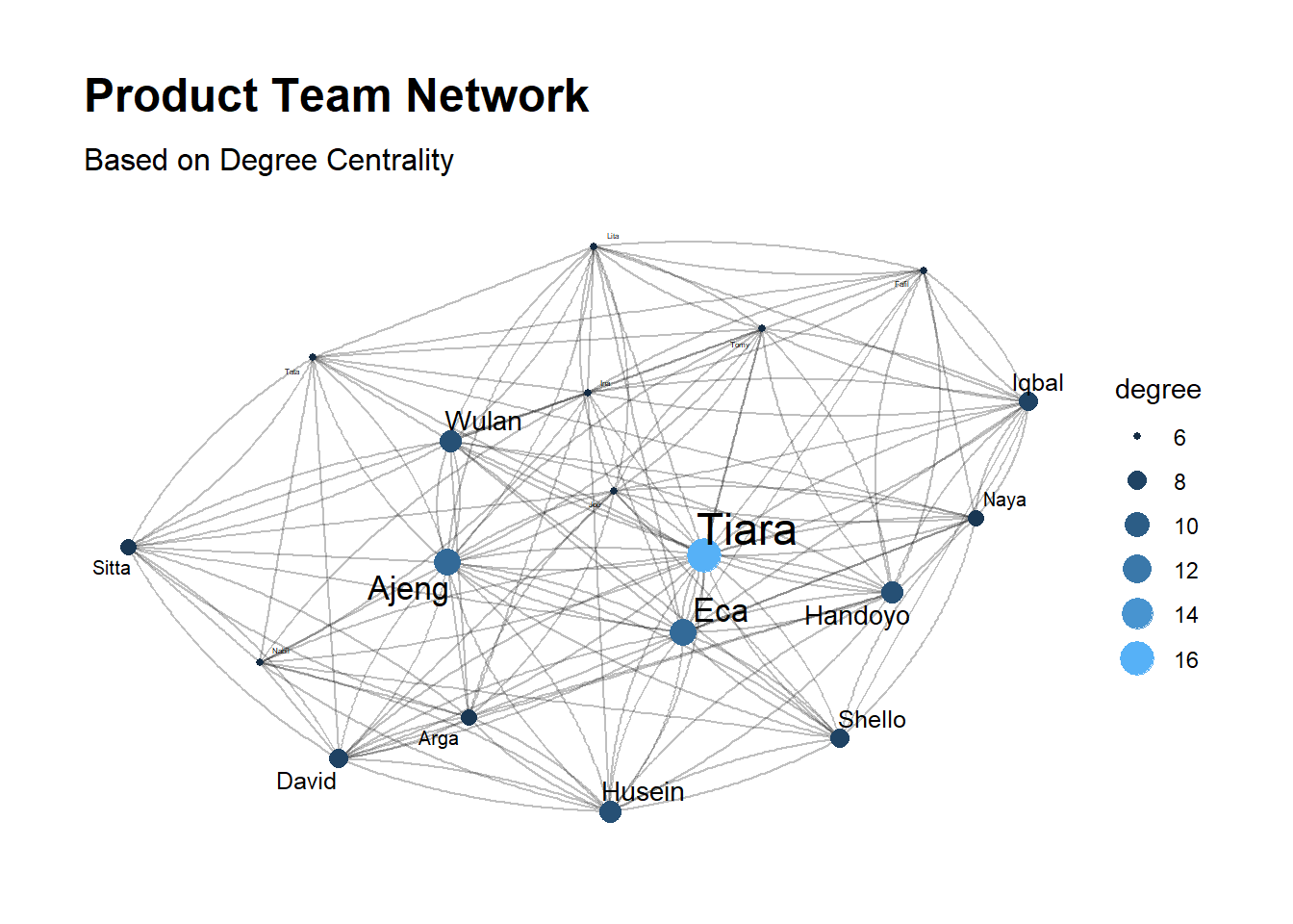
# Tiara network neighbors
g_ti <- induced.subgraph(product_net, c(2, neighbors(product_net,2)))
g_ti %>% plot(edge.arrow.size = 0.5,layout = layout.star(g_ti,center = V(g_ti)[1]))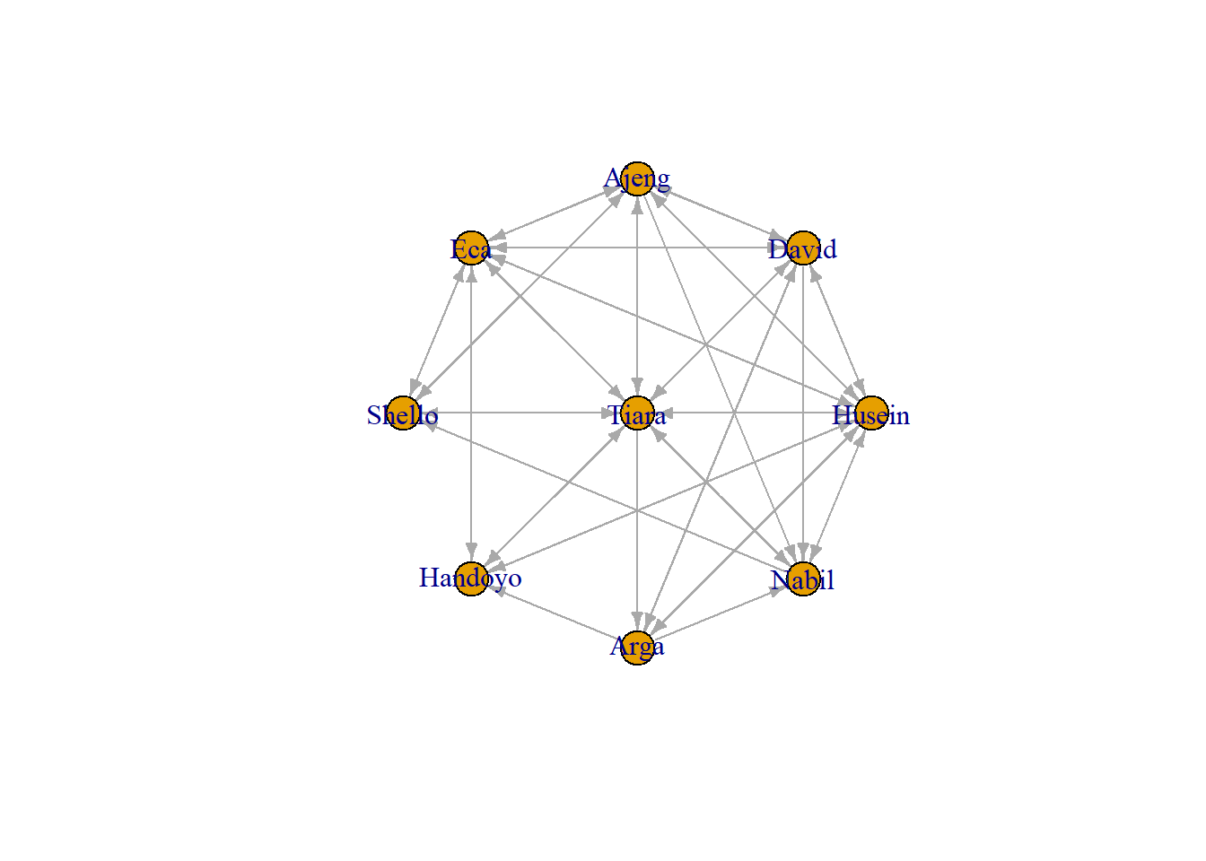
Closeness centrality
The closeness centrality of a node is the average length of the shortest path (geodesic) between the node and all other nodes in the graph. Thus the more central a node is, the closer it is to all other nodes. \[C(i) = \frac{N-1}{\sum_{j}d(j,i)}\] \(d(j,i)\) is the distance between vertices \(j\) and \(i\). This centrality divide total number of nodes minus 1(\(N-1\)) by total number of every shorthest path between one node to every node in the graph.
product_net %>%
  mutate(closeness = centrality_closeness()) %>%
  ggraph(layout = "nicely") +
  geom_edge_fan(alpha = 0.25) +
  geom_node_point(aes(size = closeness,color = closeness)) +
  geom_node_text(aes(size = closeness, label = name),
                 repel = T, show.legend = F) +
  scale_color_continuous(guide = "legend") +
  theme_graph() + labs(title = "Product Team Network",
                       subtitle = "Based on Closeness Centrality")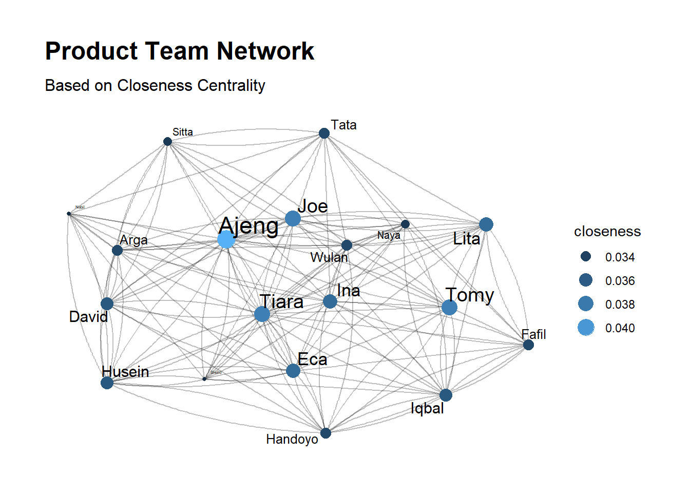
Betweenness centrality
Betweenness centrality quantifies the number of times a node acts as a bridge along the shortest path between two other nodes/groups.
\[C_{B}(v) = \sum_{ij}\frac{\sigma_{ij}(v)}{\sigma_{ij}}\]
Where \(\sigma_{ij}\) is total number of shortest paths from node \(i\) to node \(j\) and \(\sigma_{ij}(v)\) is the number of those paths that pass through \(v\)
product_net %>%
  mutate(betweenness = centrality_betweenness()) %>%
  ggraph(layout = "kk") +
  geom_edge_fan(alpha = 0.25) +
  geom_node_point(aes(size = betweenness,color = betweenness)) +
  geom_node_text(aes(size = betweenness, label = name),
                 repel = T, show.legend = F) +
  scale_color_continuous(guide = "legend") +
  theme_graph() +
  labs(title = "Product Team Network",
                       subtitle = "Based on Betweenness Centrality")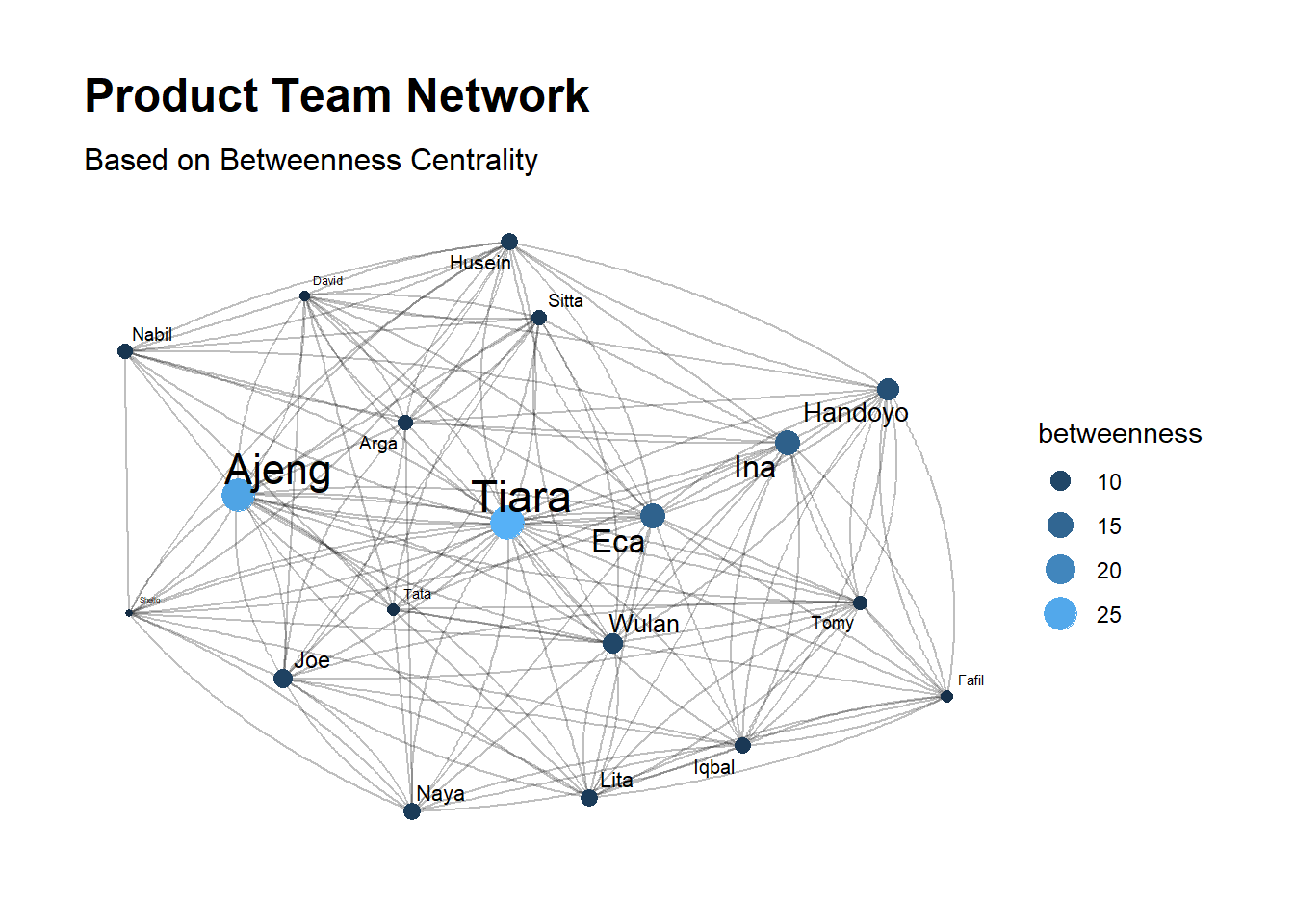
Eigenvector centrality
Eigenvector centrality is a measure of the influence of a node in a network. The relative score that is assigned to the nodes in the network is based on the concept that connections to high-scoring contributes more to the score of the node in question than equal connections to low-scoring nodes. This amazing link will help you with the calculation.
if \(A\) is the adjency matrix of a graph and \(\lambda\) is the largest eigenvalue of \(A\) and \(x\) is the corresponding eigenvector then \(Ax = \lambda x\). it can be transformed to \(x = \frac{1}{\lambda}Ax\). where \(Ax\) can be defined \(\sum_{j=1}^{N}A_{i,j}x_{j}\) therefore: \[C_{E}(i) = x_{i} = \frac{1}{\lambda}\sum_{j=1}^{N}A_{i,j}x_{j}\]
product_net %>%
  mutate(eigen = centrality_eigen()) %>%
  ggraph(layout = "nicely") +
  geom_edge_fan(alpha = 0.25) +
  geom_node_point(aes(size = eigen,color = eigen)) +
  geom_node_text(aes(size = eigen, label = name),
                 repel = T, show.legend = F) +
  scale_color_continuous(guide = "legend") +
  theme_graph() + labs(title = "Product Team Network",
                       subtitle = "Based on Eigenvector Centrality")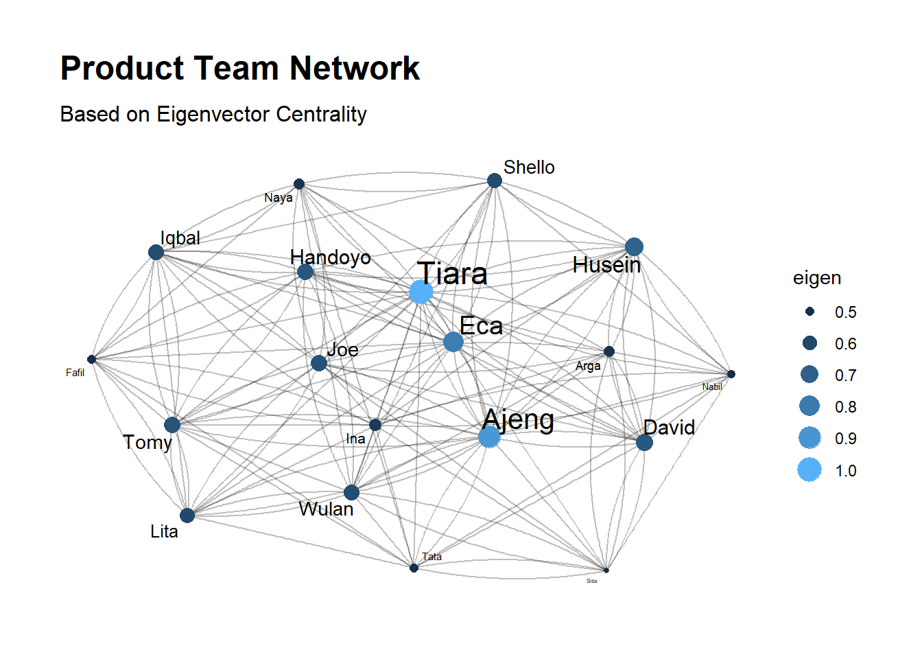
Community and Modularity
Building community in graph theory is a bit different than clustering in machine learning.igraph package implements a number of community detection methods, community structure detection algorithms try to find dense subgraphs in directed or undirected graphs, by optimizing some criteria and usually using heuristics. Community detection algorithm like group_walktrap(), group_fast_greedy(), and group_louvain() has their own way to create communities in the network. One of the common use community detection algorithm is group_walktrap(). This function tries to find densely connected subgraphs, also called communities in a graph via random walks. The idea is that short random walks tend to stay in the same community.
Modularity in the other hand, is a measure of how good the division is, or how separated are the different vertex types from each other \[Q = \frac{1}{2m}\sum_{ij}(A_{ij}-\frac{k_{i}k_{j}}{2m})\delta(c_{i},c_{j})\] here \(m\) is the number of edges, \(A_{ij}\) is the element of the \(A\) adjacency matrix in row \(i\) and column \(j\), \(k_{i}\) is the degree of \(i\), \(k_{j}\) is the degree of \(j\), \(c_{i}\) is the type (or component) of \(i\), \(c_{j}\) that of \(j\), and \(\delta(c_{i},c_{j})\) is the Kronecker delta, which returns 1 if the operands are equal and 0 otherwise. In summary, networks with high modularity have dense connections between the nodes within community but sparse connections between nodes in different community
product_net %>%
mutate(community = group_spinglass()) %>%
ggraph(layout = "nicely") +
geom_edge_fan(alpha = 0.25) +
geom_node_point(aes(color = factor(community)),size = 5, show.legend = F) +
geom_node_text(aes(label = name),repel = T) +
theme_graph() + theme(legend.position = "none") +
labs(title = "Product Team Network", subtitle = "Seperated by cluster")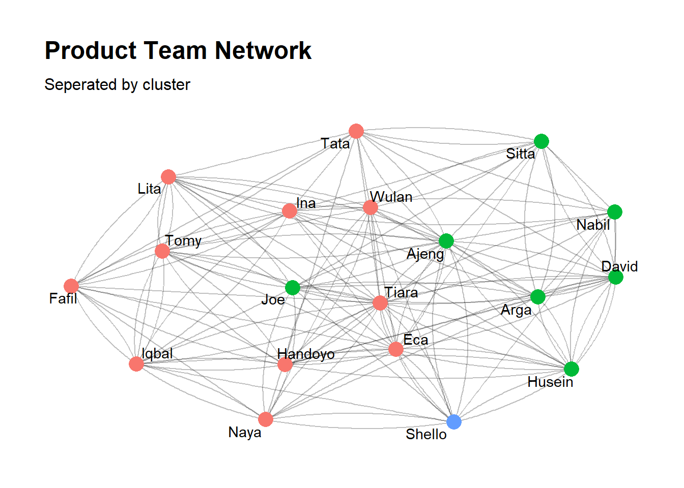 Now let’s check if this network has high or low modularity score
# first build communities using any cluster detection algorithm
cw_net <- igraph::cluster_walktrap(product_net)
modularity(cw_net)
#> [1] 0.08518007low modularity score indicates the community in the network actually don’t have much difference. There are dense connections between nodes in both communities. The community member might be different depends on what algorithm you use. you can try different algorithms and compare them using compare() function. By default, compare() returns a score by its Variance Information (method = "vi), which counts whether or not any two vertices are members of the same community. A lower score means that the two community structures are more similar
sp_net <- cluster_spinglass(product_net)
compare(comm1 = cw_net,comm2 = sp_net,method = "vi")
#> [1] 0.6614012Identify prominent user in the network
So at this point, i hope you understand the concept of graph, nodes & edges, centrality, community & modularity, and how to use it. We will move back to our Twitter network. We already convert the table_graph to data frame. Last thing we need to do is to find top account in each centrality and pull the key player
network_ego_df %>% head(5)#> name community degree_c betweenness_c closeness_c eigen
#> 1 alxmnt87 48 1 0.0000000000 0.2510361 0.0000642216
#> 2 UvACORPNET 48 1 0.0000000000 0.2510361 0.0000642216
#> 3 WSWS_Updates 48 1 0.0000000000 0.2510361 0.0000642216
#> 4 airasia_indo 48 6 0.0004356603 0.2556285 0.0007594522
#> 5 AIswinarto 48 1 0.0000000000 0.2510361 0.0000642216ey player is a term for the most influential users in the network based on different contexts. ‘Different context’ in this case is different centrality metrics. Each centrality have different use and interpretation, a user that appears in the top of most centrality will be considered as the key player of the whole network.
kp_ego <- data.frame(
  network_ego_df %>% arrange(-degree_c) %>% select(name) %>% slice(1:6),
  network_ego_df %>% arrange(-betweenness_c) %>% select(name) %>% slice(1:6),
  network_ego_df %>% arrange(-closeness_c) %>% select(name) %>% slice(1:6),
  network_ego_df %>% arrange(-eigen) %>% select(name) %>% slice(1:6)
) %>%
  setNames(c("degree","betweenness","closeness","eigen"))

kp_ego
#> degree betweenness closeness eigen
#> 1 NgajiHyung TeamAlgoritma TeamAlgoritma rykarlsen
#> 2 jasonrob_ NgajiHyung NgajiHyung chimberland
#> 3 alexajoyce jasonrob_ jasonrob_ doroii
#> 4 bodoamatewh alexajoyce shoofa_ ailourosphile
#> 5 Reuiap bodoamatewh alexajoyce megylogen
#> 6 shoofa_ Reuiap bodoamatewh haririshafaWe will exclude TeamAlgoritma from analysis because that’s our main querry, of course it has the highest centrality. “NgajiHyung” has the highest degree, betweenness, and closeness centrality, it means he has the most relation (edges) with the other nodes in the network. He also can spread information the most wide than the other. He’s the person who can spread information fastest than everyone. “rykarlsen” has the highest eigenvector centrality, he’s surrounded by important persons among the network. From the table above we can say that NgajiHyung is the key player of TeamAlgoritma ego network
Visualize Network
Let’s try to visualize the network. I’ll scale the nodes by degree centrality, and color it by community.
network_ego_df %>%
  count(community,sort = T) %>%
  head()
#> community n
#> 1 1 1257
#> 2 2 735
#> 3 3 672
#> 4 4 570
#> 5 5 561
#> 6 6 514since our network is too large (approximately 14k nodes and 15k edges), i’ll filter by only showing community 1 - 3. As the table above, community 1, 2, 3 has the highest frequency of member sequentially
options(ggrepel.max.overlaps = Inf)network_viz <- network_ego1 %>%
filter(community %in% 1:3) %>%
mutate(node_size = ifelse(degree_c >= 50,degree_c,0)) %>%
mutate(node_label = ifelse(betweenness_c >= 0.01,name,NA))plot_ego <- network_viz %>%
ggraph(layout = "stress") +
geom_edge_fan(alpha = 0.05) +
geom_node_point(aes(color = as.factor(community),size = node_size)) +
geom_node_label(aes(label = node_label),nudge_y = 0.1,
show.legend = F, fontface = "bold", fill = "#ffffff66") +
theme_graph() +
theme(legend.position = "none") +
labs(title = "TeamAlgoritma Mutual Communities",
subtitle = "Top 3 Community")plot_ego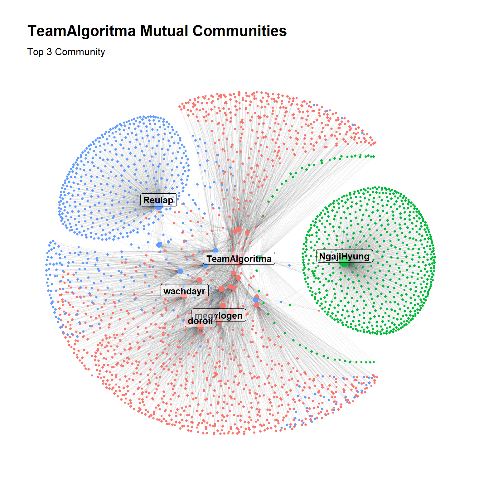
What can we get from this visualization?
This obviously doesn’t tell much of a story (we need further inspection in the data, matching it to the visualization), but it shows that the “spinglass” community detection algorithm is picking up on the same structure as “stress” layout algorithm. TeamAlgoritma as our ego appears in the middle, act as a bridge who connects all cluster. we only show user label who has high betweenness centrality value. a mushroom-shaped nodes behind them are their mutual friends who don’t follow TeamAlgoritma account. That user is our potential reader if their ‘bridge’ retweeting or mentioning something about TeamAlgoritma account. user in the same community or who close to each other maybe know each other in real life. they create their own community. The key player is in community #1 (red), which is TeamAlgoritma’s most important community because they have the most potential to spread information fast and widely.
Case 2: Activity Network
Activity network analyzes how information is spread around the network. From this analysis, we can found how something goes viral and how people interact with it. Because this network contains all forms of Twitter communication (even a single retweet), the visualization will most likely become a hairball. You will need a lot of data featuring or filtering for visualization purposes, but in the end it will be up to your preferences.
Case Objective
- Analyze Activity Network given random keyword(s) or hashtag
- Visualize the activity/information network
- find out which cluster talk about which topic regarding the keyword
- Calculate the metrics, and find out who is the
key playerin the whole conversation network
- Visualize the activity/information network
Here’s the step to do this case:
1. Gather any trending keywords or hashtag (in this case i’ll use #NewNormal)
2. Filter the data, use tweet with lots of interaction (retweet or mention)
3. Specify which column is communicating with which, then create edges df
4. Create nodes df and the network
5. Build communities, Calculate SNA metrics, and identify which user is important
6. Visualize the network
Gather tweets data
You can always choose other keywords or hashtags. in this example, i’ll use #NewNormal as the query.
womenday <- search_tweets("#InternationalWomensDay",n = 18000,include_rts = T,retryonratelimit = T)
womenday <- data.frame(lapply(womenday,as.character),stringsAsFactors = F)
it’ll take approximately 4-5 minutes and there’s a possibility of failure (sls/tls, or simply bad connection). so i provide the output in csv for us to continue the analysis.
womenday <- read.csv("data_input/SNA/womenday.csv", stringsAsFactors = F)
head(womenday,1)
#> user_id status_id created_at screen_name
#> 1 2936710628 1369203572487819264 2021-03-09 08:29:04 Minseokkyyy_799
#> text
#> 1 Saluting the brave women of Hong Kong, Thailand, and Myanmar who are bravely participating in protests in defense of democracy, and fighting against the twin authoritarian forces of establishment and patriarchy. We stand as one. #InternationalWomensDay https://t.co/qMW36VN53Q
#> source display_text_width reply_to_status_id reply_to_user_id
#> 1 Twitter for iPhone 140 NA NA
#> reply_to_screen_name is_quote is_retweet favorite_count retweet_count
#> 1 <NA> FALSE TRUE 0 2171
#> quote_count reply_count hashtags symbols urls_url urls_t.co urls_expanded_url
#> 1 NA NA <NA> <NA> <NA> <NA> <NA>
#> media_url media_t.co media_expanded_url media_type ext_media_url
#> 1 <NA> <NA> <NA> <NA> <NA>
#> ext_media_t.co ext_media_expanded_url ext_media_type mentions_user_id
#> 1 <NA> <NA> NA 578780183
#> mentions_screen_name lang quoted_status_id quoted_text quoted_created_at
#> 1 SophieMak1 en NA <NA> <NA>
#> quoted_source quoted_favorite_count quoted_retweet_count quoted_user_id
#> 1 <NA> NA NA NA
#> quoted_screen_name quoted_name quoted_followers_count quoted_friends_count
#> 1 <NA> <NA> NA NA
#> quoted_statuses_count quoted_location quoted_description quoted_verified
#> 1 NA <NA> <NA> NA
#> retweet_status_id
#> 1 1368849900171980800
#> retweet_text
#> 1 Saluting the brave women of Hong Kong, Thailand, and Myanmar who are bravely participating in protests in defense of democracy, and fighting against the twin authoritarian forces of establishment and patriarchy. We stand as one. #InternationalWomensDay https://t.co/qMW36VN53Q
#> retweet_created_at retweet_source retweet_favorite_count
#> 1 2021-03-08 09:03:42 Twitter Web App 2430
#> retweet_retweet_count retweet_user_id retweet_screen_name retweet_name
#> 1 2171 578780183 SophieMak1 Sophie Mak
#> retweet_followers_count retweet_friends_count retweet_statuses_count
#> 1 7511 453 500
#> retweet_location
#> 1
#> retweet_description
#> 1 digitally monitoring human rights abuses in <U+0001F1ED><U+0001F1F0> and elsewhere for @humanrightshku @amnesty
#> retweet_verified place_url place_name place_full_name place_type country
#> 1 FALSE <NA> <NA> <NA> <NA> <NA>
#> country_code geo_coords coords_coords bbox_coords
#> 1 <NA> c(NA, NA) c(NA, NA) c(NA, NA, NA, NA, NA, NA, NA, NA)
#> status_url
#> 1 https://twitter.com/Minseokkyyy_799/status/1369203572487819264
#> name
#> 1 <U+0001D564><U+0001D565><U+0001D552><U+0001D563><U+0001D563><U+0001D56A> <U+0001D55F><U+0001D55A><U+0001D558><U+0001D559><U+0001D565><U+0001F4AB> |||
#> location
#> 1 Lat Krabang, Bangkok
#> description
#> 1 N<U+0001D546><U+0001D54E> : <U+0001D538>P<U+0001D540>N<U+0001D542> | <U+0001D53C><U+0001D54F><U+0001D546> | <U+0001D53E><U+0001D546><U+0001D54B>7 | NC<U+0001D54B> | <U+0001D54D><U+0001D540>C<U+0001D54B><U+0001D546>N <U+2661>´<U+FF65><U+1D17><U+FF65>`<U+2661>
#> url protected followers_count friends_count listed_count
#> 1 https://t.co/7hVHIn7Stc FALSE 255 900 6
#> statuses_count favourites_count account_created_at verified
#> 1 372630 49770 2014-12-20 05:14:00 FALSE
#> profile_url profile_expanded_url account_lang
#> 1 https://t.co/7hVHIn7Stc https://twitter.com/m_itsu_ha?s=21 NA
#> profile_banner_url
#> 1 https://pbs.twimg.com/profile_banners/2936710628/1585838104
#> profile_background_url
#> 1 http://abs.twimg.com/images/themes/theme5/bg.gif
#> profile_image_url
#> 1 http://pbs.twimg.com/profile_images/1251526099470696450/alWvrXec_normal.jpgBuild edges, nodes, and graph dataframe
mentions_screen_name column contains user screen_name we interact with. it’ll be our “to” column in edges. however, by default the column is list type (that i convert to character). We need to remove unused string first. Here’s a function to remove all symbols except letter, number and comma ’ , ’. it also remove first letter in the string (c in our case)
mention_clean <- function(x){
  if(grepl(",",x) == TRUE){
    gsub('^.|[^[:alnum:][:blank:]_,?&/\\-]',"",x)
  } else{
    x
  }
}
then we simply apply it to the column
# apply mention_clean function to mentions_screen_name column using sapply()
edge_nn <- womenday %>%
  select(screen_name,is_retweet,mentions_screen_name) %>%
  mutate(mentions_screen_name = sapply(mentions_screen_name,mention_clean))

# specify interaction type
edge_nn <- edge_nn %>%
  mutate(type = ifelse(is_retweet == TRUE,"retweet","mention"))

# seperate value in mention_screen_name by comma
edge_nn <- edge_nn %>%
  select(screen_name,mentions_screen_name,type) %>%
  separate_rows(mentions_screen_name,sep = ",") %>%
  setNames(c("from","to","type")) %>%
  count(from,to,type)

# create nodes dataframe by unique value in both edges column
nodes_nn <- data.frame(V = unique(c(edge_nn$from,edge_nn$to)),
                        stringsAsFactors = F)

# build graph data
network_nn <- graph_from_data_frame(d = edge_nn, vertices = nodes_nn, directed = T) %>%
  as_tbl_graph()

# create community, calculate centrality and remove loop edge
set.seed(123)
network_nn <- network_nn %>%
  activate(nodes) %>%
  mutate(community = tidygraph::group_infomap(),
         degree = centrality_degree(),
         between = centrality_betweenness(),
         closeness = centrality_closeness(),
         eigen = centrality_eigen()) %>%
  activate(edges) %>%
  filter(!edge_is_loop())

network_act_df <- as.data.frame(network_nn %>% activate(nodes))
Identify a prominent person in the network
Key players in the ego network and activity network have different interpretation. In this case, the key player will be considered as a person who makes this specific keyword viral. We also can identify which person whose opinions are widely agreed upon by others.
kp_activity <- data.frame(
  network_act_df %>% arrange(-degree) %>% select(name) %>% slice(1:6),
  network_act_df %>% arrange(-between) %>% select(name) %>% slice(1:6),
  network_act_df %>% arrange(-closeness) %>% select(name) %>% slice(1:6),
  network_act_df %>% arrange(-eigen) %>% select(name) %>% slice(1:6)
) %>% setNames(c("degree","betweenness","closeness","eigen"))

kp_activity
#> degree betweenness closeness eigen
#> 1 womeninstemSA ABVPVoice womeninstemSA NA
#> 2 AbhiTha84389697 nowthisnews AbhiTha84389697 abbasali210
#> 3 ir_child BedeleBuno ir_child lindsay_joker
#> 4 YuliyaInopinaPR EBCharts YuliyaInopinaPR 4freedominiran2
#> 5 Mona3Dimaging DelhiAipc Mona3Dimaging nowthisnews
#> 6 Wackelkasper VijayPU00200338 Wackelkasper redfishstreamWe got interesting results here. almost every top centrality has a different account. Ignore NA in eigen centrality, it because we calculate centrality from missing directed graph. It means every top user is great in their own ‘job’ on the network. From the table above, “womeninstemSA” grab my attention the most. he appears in 2 centrality Thus we can conclude she is the key player in #InternationalWomensDay Twitter activity network. Let’s see his tweets
womenday %>%
  filter(screen_name == "womeninstemSA") %>%
  arrange(-retweet_count) %>%
  select(created_at,text,retweet_count) %>%
  head(3)
#> created_at
#> 1 2021-03-09 08:09:58
#> 2 2021-03-09 08:08:24
#> 3 2021-03-09 08:00:59
#> text
#> 1 My commitment to refuse invitations to academic conferences with all-male lineup is in its 5th year. I stick to this & I encourage other scientists to join. The fight for equality is far from over.\n#InternationalWomensDay \n#WomenInScience #WomenInSTEM
#> 2 Buckle in for an #InternationalWomensDay<U+0001F9F5>, highlighting the work of women in science. \nTo start: Katie Bouman, who led the creation of an algorithm that helped capture the first ever image of a black hole. Here she is speaking about the breakthrough in 2019 #IWD2021 #womeninstem https://t.co/0KmjkfFHD1
#> 3 As women in #STEM, we #ChooseToChallenge stereotypes, gender bias, and discrimination and celebrate #InternationalWomensDay \n\n#IWD2021 #WomenInSTEM @BTS_twt https://t.co/86WmNT7aaH
#> retweet_count
#> 1 200
#> 2 110
#> 3 67Visualize network
let’s try to visualize the network. the network consist of 45k+ nodes and 42k+ degree. we need to filter it otherwise it’ll be just hairball of nodes and edges. here i just plot top 3 community and filter the label by nodes with degree centrality >= 3 or betweenness centrality >= 100. The edges color are separated by interaction type.
network_nn %>%
  activate(nodes) %>%
  mutate(ids = row_number()) %>%
  filter(community %in% 1:3) %>%
  arrange(community,ids) %>%
  mutate(node_label = ifelse(degree >= 3 | between >= 8,name,"")) %>%
  mutate(node_size = ifelse(degree >= 3 | between >= 8,degree,0)) %>%
  ggraph(layout = "linear", circular = T) +
  geom_edge_arc(alpha = 0.05, aes(col = as.factor(type), edge_width = n*0.5)) +
  # geom_node_label(aes(label = node_label, size = node_size),repel = T,
  #                show.legend = F, fontface = "bold", label.size = 0,
  #                segment.colour="slateblue", fill = "#ffffff66") +
  ggrepel::geom_label_repel(aes(x = x, y = y, label = node_label,size = node_size),
                            fontface = "bold", label.size = 0,show.legend = F,
                            segment.colour="slateblue", fill = "#ffffff66") +
  labs(title = "Twitter Activity Network #InternationalWomensDay",
       subtitle = "Retweets and mention between 3 top communities") +
  theme_graph() +
  guides(edge_width = F,
         edge_colour = guide_legend(title = "Tweet Type",
                                    override.aes = list(edge_alpha = 1))) +
  theme(legend.position = "bottom")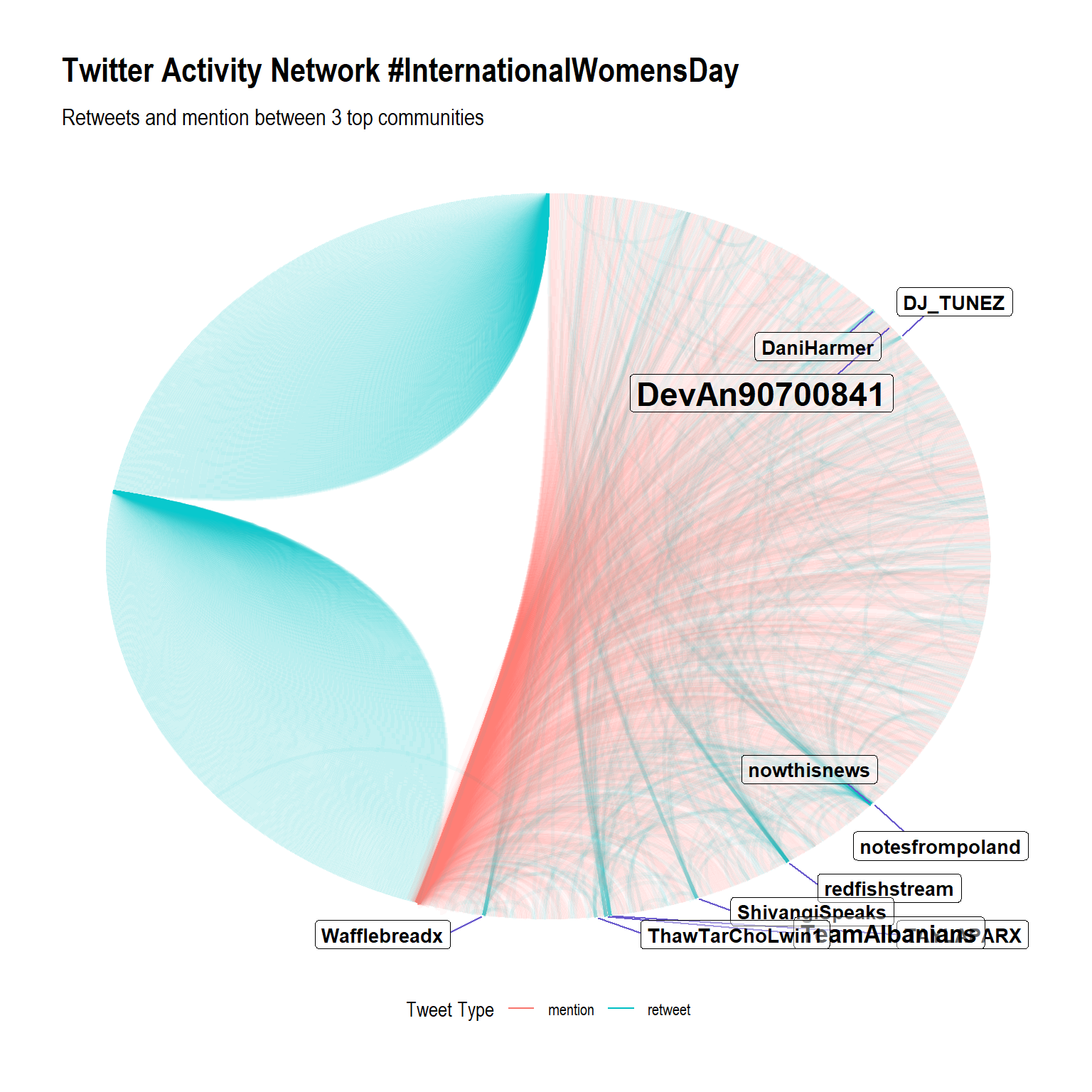
What can we get from this visualization?
First, lets see this table
network_act_df %>%
  arrange(-degree) %>%
  group_by(community) %>%
  slice(1:5)
#> # A tibble: 28,362 x 6
#> # Groups: community [9,461]
#> name community degree between closeness eigen
#> <chr> <int> <dbl> <dbl> <dbl> <dbl>
#> 1 DevAn90700841 1 4 0 4.93e-10 0.00217
#> 2 BFujer 1 2 0 4.92e-10 0.0276
#> 3 LAHSGwalior 1 2 0 4.92e-10 0.0276
#> 4 RaviBhai2705 1 2 2 4.92e-10 0.0276
#> 5 TeamAlbanians 1 2 21 4.92e-10 0.0280
#> 6 GentlemanShrink 2 2 0 4.93e-10 0.000722
#> 7 __crbr 2 1 0 4.92e-10 0.000000947
#> 8 __malea__ 2 1 0 4.92e-10 0.000000947
#> 9 _chxline 2 1 0 4.92e-10 0.000000947
#> 10 _dnbss 2 1 0 4.92e-10 0.000000947
#> # ... with 28,352 more rowsNow we can identify which person belongs to which community based on highest degree. The plot is arranged by community and id (row number), so user in the same community are placed near to each other. community #1 (highest community by frequency) is the only community with 2 interaction types (you can detect community in the plot by add geom_node_label() and set the aes color to community. lots of them are retweeting (or quoting) “DevAn90700841” tweet, and the others mentioning to each other. Users in community #2 and #3 are just retweeting each other, or maybe some of them make a quote tweet that also goes viral. I can conclude that the top 3 community (by highest frequency) in Twitter activity network is well separated by its tweet types (interaction types). maybe there’s another interesting insight in another community since it creates fewer accounts by each community.
Additional business case: Competition network
Competition network gathers all person/user who has connection to specific official account. The main idea is mapping the whole network of accounts in the same industry. for example, we want to see marketing competition in Indonesian private colleges. We gather all of their followers and from that follower, gather all their following. Build community and calculate the metrics, thus we will get important persons who has information from all competing accounts. we also can found which community is a potential ‘unreached’ market to several companies and how to reach them.
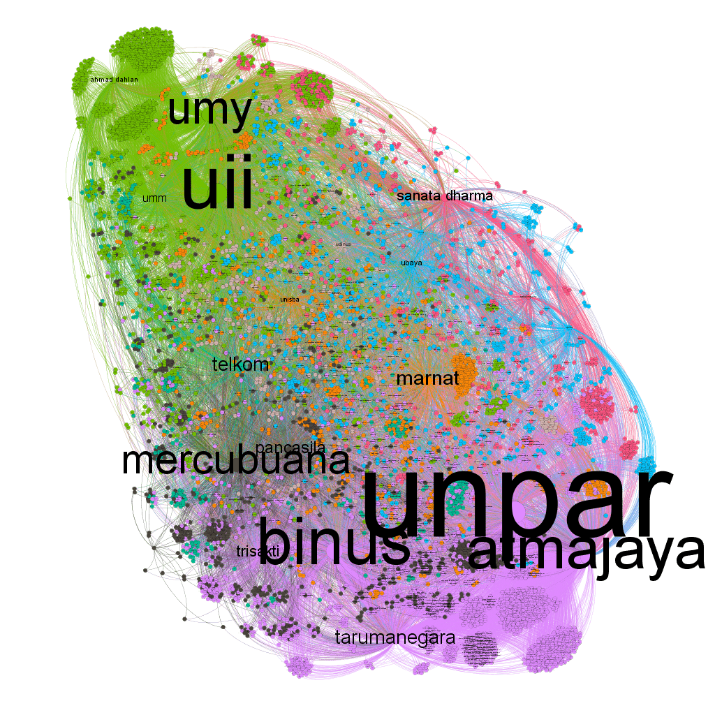
The graph above shows 21 Indonesian private college Instagram admission of new student network. The network is separated by 3 community, green for Muslim college, purple for Catholic/Christian college, and fuzzy cluster in the middle is what we can say as a ‘neutral’ college. We can conclude that these days people still looking for education based on their religion. Let’s say we’re a social media analyst from Binus, then we can find out how to reach UII/UMY/UMM cluster based on important person in their community (endorsement). It will give Binus a lot of engagement right?
Well, the problem is Twitter rate limitation makes it impossible to do this analysis in a short time. So i’ll tell you how to do it. It’s pretty simple, but takes a loong time:
- Select several accounts in the same industry
- Gather all of their followers
- From the follower, gather all of their following
- Filter to active user only (if possible)
- Build a network, create community and centrality
- Identify prominent user based on your case
- Visualize
Case Objectives:
- Analyze Competition Network from (for example) @kfc_id, @mcd_id, @wendys, @phd account
- Visualize the whole competition network
- Identify fanbase cluster in each account
- Calculate the metrics, and find out who is the
key playerin the whole network
- Visualize the whole competition network
Reference
SNA with R:
- Rtweet homepage
- Tidygraph introduction
- Tidygraph introduction 2
- R Twitter network example (my main reference)
- Various R packages for SNA
- igraph manual pages
- R-graph gallery
Thank you !


 More details
 More details
Share this post
Twitter
Facebook
LinkedIn